Variational Method

Recall that in quantum mechanics, the ground state energy can be defined variationally as

\[ E_{0}=\min _{\psi} \frac{\langle\psi|\hat{H}| \psi\rangle}{\langle\psi \mid \psi\rangle} \]

To obtain an exact result, the minumum is taken over the full Hilbert space. But we can obtain an upper bound on the \(E_0\) by a “few” parameter ansatz \(\psi=\left|g_{1,}, g_{2}, \cdots\right\rangle\), where \(g_i\) are parameters. For example, we could approximate \(\psi\) by the Gaussian \(\langle r|g\rangle=e^{-\frac{1}{2} g r^{2}}\) with just one parameter \(g\). Then,

\[ E_0\leq \frac{\langle g|\hat{H}|g\rangle}{\langle g|g\rangle} \]

The \(|g\rangle\) obtained in this way is in this sense the “best” approximation to \(\left|E_{0}\right\rangle\) in the Hilbert subspace \(\mid \{ g\} \rangle\).

We can do something similar in statistical physics.

Given \(T, H\), we define the free-energy of an arbitrary distribution \(p\) by

\[\begin{split} \begin{aligned} F[p] & \equiv \sum p_{\mu}\left(H[\mu]+k_B T \ln \left(p_{\mu}\right)\right) \\ & =\langle H\rangle_p-T S[p] \end{aligned} \end{split}\]

where we’ve used the Gibbs entropy

\[ S[p]=- k_B \sum_{\mu} p_{\mu} \log \left(p_{\mu}\right) \]

Recall that the Boltzmann distribution \(\hat p\equiv \frac{1}{Z_{\beta}} e^{-\beta H}=e^{-\beta (H-F_0)}\) minimizes the functional \(F\) (Because \(\hat p\) maximizes the Gibbs entropy subject to \(\langle E\rangle\)). Therefore, we have the inequality

\[ F[p] \geq F\left[\hat p\right] \equiv F_{0} \]

Given a few-parameter ansatz \(p_{\mu}(g)\), we can then define our best approximation as

(10)\[ \min_{g} F[p(g)] \geq F_{0} \]

and use \(p(g)\) to compute approximate observables.

Note that there is a simple way to see that () is true. First, the difference in approximate and true free energy is

(11)\[ \beta\left(F[p(g)]-F_{0}\right)=\beta\left[\langle H\rangle_{p(g)}-F_{0}\right]-S[p(g)]/k_B =\beta\left[\langle H\rangle_{p(g)}-F_{0}\right]+\langle \ln(p(g))\rangle_{p(g)} \]

The first term can be rewritten after noting that the structure of the true distribution, \(\hat p=e^{-\beta (H-F_0)}\), allows us to write \(\langle \hat p \rangle_{p} = -\beta (\langle H \rangle_{p} - F_0)\). Thus, we obtain

\[ \beta\left(F[p(g)]-F_{0}\right)=-\langle \ln(\hat p)\rangle_{p(g)}+\langle \ln(p(g))\rangle_{p(g)} =D_{KL}\left(p(g) \| \hat p\right) \]

showing that the difference between the approximate and true free energy is proportional to the “KL” divergence

\[ D_{K L}(P \| Q)= \sum P_{i} \ln \left(\frac{P_{i}}{Q_{i}}\right) \geq 0 \]

which is non-negative (see Shannon entropy lecture, eq. (2)).

It is convenient to parameterize \(p(g)\) as a Boltzmann distribution corresponding to a fictitious Hamiltonian \(H_g\),

\[ p(g) \equiv \frac{1}{Z_{g}} e^{-\beta H_{g}}\;. \]

Consider, for example, the generalized Ising Hamiltonian

\[H=-J \sum_{\langle i, j\rangle} \sigma_{i} \sigma_{j}\]

where the notation \(\langle i, j\rangle\) indicates that sites \(i\) and \(j\) are in contact (i.e. they are nearest neighbors) and each pair is only counted once. We might then choose \(H_{g}=-g \sum_{i} \sigma_{i}\), where \(g\) is a parameter we will adjust. In terms of \(H_g\), we have

\[ F[p(g)]=\sum_{\mu} \frac{e^{-\beta H_{g}(\mu)}}{Z_{g}}\left(H(\mu)+\frac{1}{\beta} \ln \left(\frac{e^{-\beta H_{g}(\mu)}}{Z_{g}}\right)\right) \]

Defining \(\quad e^{-\beta F_{g}}\equiv Z_{g}= \sum_{\mu} e^{-\beta H_{g}(\mu)}\quad\left(F_{g} \neq F[p(g)] !\right)\), we have

\[ F[p(g)]=\langle H\rangle_{g}-\left\langle H_{g}\right\rangle_{g}+F_{g} \]

The lower bound

\[ F[p(g)]-F_{0}=F_{g}-F_{0}+\langle H\rangle_{g}-\left\langle H_{g}\right\rangle_{g} \geq 0 \]

is called the “Gibbs’s inequality”. It can be rewritten as

\[\begin{split} \begin{aligned} -\frac{1}{\beta}\left(\ln \left(Z_{g}\right)-\right. & \ln (Z))+\langle H\rangle_{g}-\left\langle H_{g}\right\rangle_{g} \geqslant 0 \\ & \ln (Z) \geqslant \ln (Z_g)+\beta\left(\langle H_g\rangle_{g}-\langle H\rangle_{g}\right) \end{aligned} \end{split}\]

Let’s try this for

\[\begin{split} \begin{aligned} H & =-J \sum_{\langle i, j\rangle} \sigma_{i} \sigma_{j}, \\ H_{g} & =-g \sum_{i}^{N} \sigma_{i}, \quad \text { "Mean field ansatz", where g="Mean Field". } \end{aligned} \end{split}\]

We need to compute \(Z_{g},\left\langle H_{g}\right\rangle_{g},\langle H\rangle_{g}\)

\[\begin{split} \begin{aligned} & Z_{g}=\left(e^{\beta g}+e^{-\beta g}\right)^{N}=[2 \cosh (\beta g)]^{N}\equiv z_g^N \\ & F_{g}=-\frac{1}{\beta} N \ln[2 \cosh (\beta g)] \\ & \left\langle H_{g}\right\rangle_g=-g\left \langle \sum_{i} \sigma_{i}\right\rangle_{g} \end{aligned} \end{split}\]

which depends on the mean magnetization \(m_g\) under the fictitious Hamiltonian,

\[ m_{g}\equiv \langle \sigma_i \rangle_g= N^{-1}\left \langle \sum_{j} \sigma_{j}\right\rangle_{g}=(Ng)^{-1}\partial_{\beta} \ln \left(Z_{g}\right)=\tanh (\beta g)\;. \]

And crucially, because under \(p(g)\) the different spins are uncorrelated,

\[\begin{split} \begin{aligned} & p_{g}\left(\sigma_{1}, \sigma_{2}, \ldots\right)=p_{g}\left(\sigma_{1}\right) p_{g}\left(\sigma_{2}\right) \ldots \\ &=\prod_{i}\underbrace{\left(\frac{e^{-\beta g \sigma_{i}}}{z_g}\right)}_{p_{g}\left(\sigma_{i}\right)} \end{aligned} \end{split}\]

we obtain for the \(p(g)\) averaged energy

\[\begin{split} \langle H\rangle_{g}=-J \sum_{\langle i, j\rangle}\left\langle\sigma_{i} \sigma_{j}\right\rangle_{g}=-J \sum_{\langle i, j\rangle}\left\langle\sigma_{i}\right\rangle_{g}\left\langle\sigma_{j}\right\rangle_{g}\\ =-J \sum_{\langle i, j\rangle} m_g^2=-J \sum_{\langle i, j\rangle} \tanh ^{2}(\beta g)=\frac{N \zeta}2 \tanh ^{2}(\beta g) \end{split}\]

where \(\zeta\) is the number of nearest neighbors each spin has - the so-called coordination number.

Putting it all together

\[\begin{split} \begin{aligned} & F[p(g)]=\langle H\rangle_{g}-\langle H_g\rangle_{g}+F_{g} \\ & =-J \frac{N \zeta}{2} m_{g}^{2}+N g m_{g}-\frac{1}{\beta} N \ln [2 \cosh (\beta g)] \end{aligned} \end{split}\]

Now, finally, we minimize (\(m_{g}^{\prime}=\partial_{g} m_{g}\)):

\[\begin{split} \begin{aligned} & \partial_{g} F[p(g)]=N\partial_{g} \left[-J \frac{\zeta}{2} m_{g}^{2}+g m_{g}-\frac{1}{\beta} \ln (\cosh (\beta g))\right] \\ &=N\left[-J \zeta m_{g} m_{g}^{\prime}+g m_{g}^{\prime}+m_{g}-m_{g}\right]=0 \end{aligned} \end{split}\]

So, we obtain the self-consistency condition

\[ g=J \zeta \cdot m_{g}=J \cdot \zeta \cdot \tanh (\beta g) \;, \]

which has a simple physical interpretation: in \(H=-J\sum_{\langle i, j\rangle} \sigma_{i} \sigma_{j}\), each \(\sigma_{i}\) sees “on average” a field \(J \zeta \langle \sigma_i\rangle_g=J \zeta m_g\) induced by its neighors - suggesting \(H\approx -J \zeta m_g\sum_i \sigma_i\). Since \(H_{g}=-g \sum_i \sigma_{i}\), the condition is \(g=J \zeta m_g\).

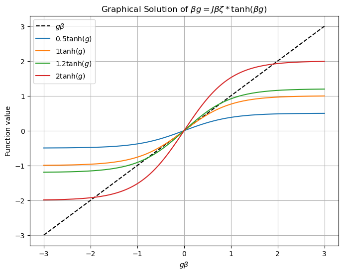
We can solve \(g=J \zeta \tanh (\beta g)\) analytically for small \(g\) :

\[ g=J \zeta \beta g\left(1-\frac{1}{3}(\beta g)^{2}\right)+\cdots \]

Solution \(1: g=0 . \longrightarrow m_{g}=0\)

But for \(J \zeta \beta>1\),

\[ 1=J \zeta \beta\left(1-\frac{1}{3}(\beta g)^{2}\right) \]

Solution 2: \(\beta g= \pm \sqrt{3\left(1-\frac{1}{J \zeta \beta}\right)}\)

\[ m_{g}= \pm \sqrt{3\left(1-\frac{1}{J \zeta \beta}\right)} \]

For \(J \zeta \beta>1\), it can be verified this is lower-F solution: symmetry breaking!

Graphical Solution of

\[ \beta g=J \beta \zeta \tanh (\beta g) \]

Show code cell source Hide code cell source

import numpy as np
import matplotlib.pyplot as plt

# Define the parameters for multiple J values
J_values = [0.5, 1, 1.2, 2]
g_values = np.linspace(-3, 3, 400)  # Range of g values for plotting

# Plotting for multiple J values
plt.figure(figsize=(8, 6))
plt.plot(g_values, g_values, label='$g\\beta$', linestyle='--', color='black')

for J in J_values:
    tanh_function = J * np.tanh(g_values)
    plt.plot(g_values, tanh_function, label=f'${J} \\tanh(g)$')

plt.title('Graphical Solution of $\\beta g = J \\beta \\zeta * \\tanh(\\beta g)$')
plt.xlabel('$g\\beta$')
plt.ylabel('Function value')
plt.legend()
plt.grid(True)
plt.show()

Is this variational approximation good?

It knows about the lattice and dimensions \(D=1,2,3\) only through coordinatione number \(\zeta\). e.g., for square lattice \(\quad \zeta=2 D \)

But we know that the exact solution of 1D Ising model does not have symmetry breaking: the variational result is bad in 1D. On the other hand, if \((D, \zeta) \rightarrow \infty\), you can verify \(F[p(g)]\) is identical to the exact result of the all-to-all model: it is good in large \(D\) and large \(\zeta\).

For \(D=2,3\), the accuracy is intermediate; it correctly predicts symmetry breaking but doesn’t get \(T_{c}\) or \(m \sim\left|T-T_{c}\right|^{\beta}\) quantitatively right.