Molecular Dynamics Simulation of Thermalization

Introduction

This code simulates the thermalization of a system of particles undergoing elastic collisions. It models a 2D gas where particles are initially divided into two populations:

• Hot particles with a higher initial temperature

• Cold particles with a lower initial temperature

As the simulation progresses, particles collide and exchange energy, leading to thermal equilibration. The key observables in this simulation include:

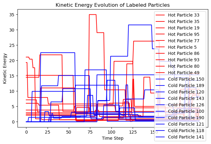
1. Kinetic energy evolution of labeled particles

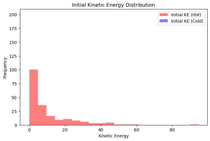
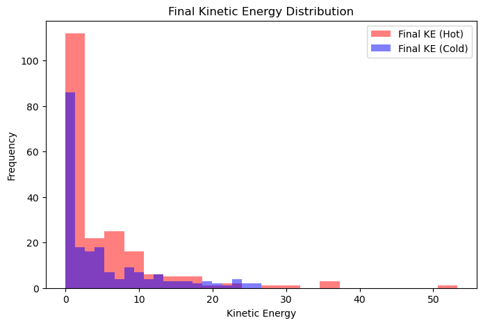
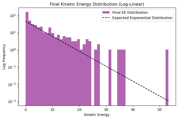
2. Histogram of kinetic energy distributions before and after thermalization (now with a log-linear plot)

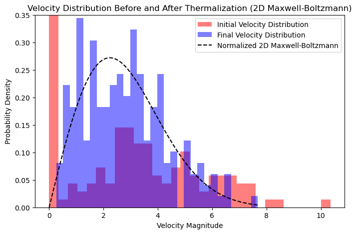
3. Velocity distributions before and after thermalization, compared to the normalized 2D Maxwell-Boltzmann distribution

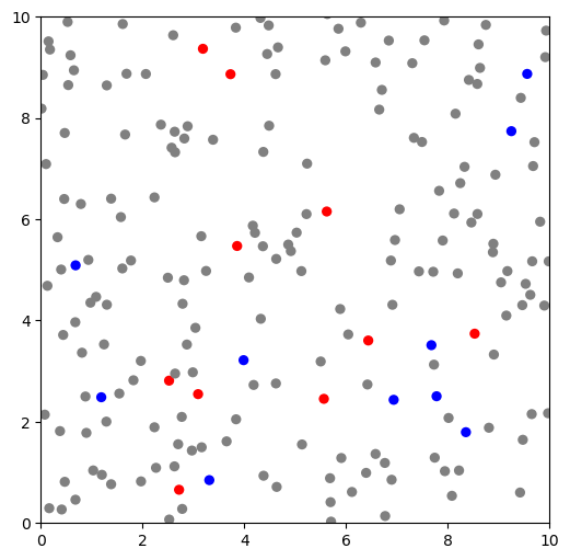
4. An animated visualization of particle dynamics (optimized for inline rendering in Jupyter Book)

Physical Model

Each particle follows Newtonian mechanics, moving freely until it collides with a wall or another particle.

Hard-Sphere Collision Model

Particles are modeled as hard spheres, meaning their interactions follow elastic collision laws:

• Momentum and kinetic energy are conserved.

• Collisions with walls are perfectly elastic.

• Particle-particle collisions are explicitly handled using momentum and energy conservation equations.

Initial Conditions

• Particles are assigned random positions within a box.

• Half of the particles are initialized with higher kinetic energy (hot particles), while the other half have lower kinetic energy (cold particles).

• A small subset of particles is labeled for tracking.

Thermalization Process

As time progresses, the energy distribution evolves due to collisions, approaching a Boltzmann distribution. The final kinetic energy distribution should follow an exponential distribution, characteristic of a system in thermal equilibrium.

Implementation Details

• Elastic collisions are detected and handled via velocity updates.

• Hard-sphere interactions are included to ensure realistic thermalization.

• Kinetic energy tracking is performed for labeled hot and cold particles.

• Animation subsampling is implemented to reduce memory overhead.

• Histograms show the initial and final kinetic energy distributions, now also in a log-linear plot.

• Velocity distributions are plotted and compared to the properly normalized 2D Maxwell-Boltzmann distribution.

Visualization and Outputs

1. Inline animation of particle motion (compatible with Jupyter Book, avoids external windows).

2. Time series plots of kinetic energy for labeled particles (rendered inline in Jupyter Book).

3. Histograms of kinetic energy distributions before and after equilibration, including a log-linear plot.

4. Velocity distributions before and after thermalization, with an overlay of the normalized 2D Maxwell-Boltzmann distribution.

import numpy as np
import matplotlib.pyplot as plt
import matplotlib.patches as patches
import matplotlib.animation as animation
from IPython.display import HTML
import matplotlib
#matplotlib.use('Agg') 

# Simulation parameters
N = 200  # Total number of particles
m = 20    # Number of labeled particles
L = 10.0 # Box size
T_hot = 10.0  # Temperature of hot particles
T_cold = 0.0  # Temperature of cold particles
dt = 0.01 # Time step
steps = 200  # Increased number of simulation steps
subsample_rate = 3  # Reduce memory by updating animation every 10 steps
radius = 0.1  # Particle radius for collisions

# Initialize particle properties
np.random.seed(42)
pos = np.random.rand(N, 2) * L  # Random positions

# Ensure particles are not overlapping initially
for i in range(N):
    for j in range(i + 1, N):
        while np.linalg.norm(pos[i] - pos[j]) < 2 * radius:
            pos[j] = np.random.rand(2) * L  # Relocate if overlapping

# Divide population into hot and cold
half_N = N // 2
vel = np.zeros((N, 2))
vel[:half_N] = np.random.randn(half_N, 2) * np.sqrt(T_hot)  # Hot particles
vel[half_N:] = np.random.randn(half_N, 2) * np.sqrt(T_cold)  # Cold particles

velini = vel.copy()

# Choose labeled particles from both groups
labeled_hot = np.random.choice(range(half_N), m//2, replace=False)
labeled_cold = np.random.choice(range(half_N, N), m//2, replace=False)
labeled_indices = np.concatenate((labeled_hot, labeled_cold))

# Track the kinetic energy of labeled particles
time_series = {i: [] for i in labeled_indices}

def compute_collisions(pos, vel, L):
    """Detects and handles collisions with walls and between particles."""
    for i in range(N):
        for dim in range(2):
            if pos[i, dim] <= 0 or pos[i, dim] >= L:
                vel[i, dim] *= -1  # Elastic collision with walls
    
    # Particle-particle collisions
    for i in range(N):
        for j in range(i + 1, N):
            dist = np.linalg.norm(pos[i] - pos[j])
            if dist < 2 * radius:  # Hard-sphere collision condition
                normal = (pos[j] - pos[i]) / dist
                v1n = np.dot(vel[i], normal)
                v2n = np.dot(vel[j], normal)
                v1t = vel[i] - v1n * normal
                v2t = vel[j] - v2n * normal
                vel[i] = v2n * normal + v1t  # Swap normal velocity components
                vel[j] = v1n * normal + v2t
    return vel

# Visualization setup
fig, ax = plt.subplots(figsize=(6, 6))
ax.set_xlim(0, L)
ax.set_ylim(0, L)
colors = ['red' if i in labeled_hot else 'blue' for i in labeled_indices]
particles = [plt.Circle(pos[i], radius, fc=colors[labeled_indices.tolist().index(i)] if i in labeled_indices else 'gray') for i in range(N)]
for p in particles:
    ax.add_patch(p)

def update(frame):
    """Update particle positions in animation with subsampling."""
    global pos, vel
    for _ in range(subsample_rate):  # Advance simulation subsample_rate steps per frame
        pos += vel * dt  # Update positions
        vel = compute_collisions(pos, vel, L)  # Handle collisions
        for i in labeled_indices:
            kinetic_energy = 0.5 * np.linalg.norm(vel[i])**2
            time_series[i].append(kinetic_energy)
    for i, p in enumerate(particles):
        p.set_center(pos[i])
    return particles

ani = animation.FuncAnimation(fig, update, frames=steps // subsample_rate, blit=False, interval=10)
HTML(ani.to_jshtml())  # Ensure inline animation in Jupyter Book

Once Loop Reflect

# Plot kinetic energy time series inline
%matplotlib inline
plt.figure(figsize=(8, 5))
for i in labeled_hot:
    plt.plot(time_series[i], color='red', label=f'Hot Particle {i}')
for i in labeled_cold:
    plt.plot(time_series[i], color='blue', label=f'Cold Particle {i}')
plt.xlabel('Time Step')
plt.ylabel('Kinetic Energy')
plt.title('Kinetic Energy Evolution of Labeled Particles')
plt.legend()
plt.show()

# Plot the kinetic energy histograms inline
plt.figure(figsize=(8, 5))
plt.hist(velini[:half_N].flatten()**2, bins=20, alpha=0.5, color='red', label='Initial KE (Hot)')
plt.hist(velini[half_N:].flatten()**2, bins=20, alpha=0.5, color='blue', label='Initial KE (Cold)')
plt.xlabel('Kinetic Energy')
plt.ylabel('Frequency')
plt.title('Initial Kinetic Energy Distribution')
plt.legend()
plt.show()

plt.figure(figsize=(8, 5))
plt.hist(vel[:half_N].flatten()**2, bins=20, alpha=0.5, color='red', label='Final KE (Hot)')
plt.hist(vel[half_N:].flatten()**2, bins=20, alpha=0.5, color='blue', label='Final KE (Cold)')
plt.xlabel('Kinetic Energy')
plt.ylabel('Frequency')
plt.title('Final Kinetic Energy Distribution')
plt.legend()
plt.show()

%matplotlib inline
# Plot the kinetic energy histogram on a log-linear scale
plt.figure(figsize=(8, 5))
ke_values = np.concatenate((vel[:half_N].flatten()**2, vel[half_N:].flatten()**2))
plt.hist(ke_values, bins=50, alpha=0.6, color='purple', label='Final KE Distribution', log=True)

# Expected final distribution (Exponential distribution of KE over thermal energy)
T_final = (T_hot + T_cold) / 2
ke_expected = np.linspace(0, max(ke_values), 100)
exp_distribution = (1 / T_final) * np.exp(-ke_expected / T_final) * len(ke_values) * np.mean(np.diff(ke_expected))
plt.plot(ke_expected, exp_distribution, 'k--', label='Expected Exponential Distribution')

plt.xlabel('Kinetic Energy')
plt.ylabel('Log Frequency')
plt.title('Final Kinetic Energy Distribution (Log-Linear)')
plt.legend()
plt.show()

%matplotlib inline
import numpy as np
import matplotlib.pyplot as plt
from scipy.stats import maxwell

# Compute velocity magnitudes before and after thermalization
vel_initial = np.linalg.norm(velini, axis=1)
vel_final = np.linalg.norm(vel, axis=1)

# Properly normalized 2D Maxwell-Boltzmann distribution
T_final = (T_hot + T_cold) / 2  # Final temperature assumption
v_range = np.linspace(0, np.max(vel_final), 100)
mb_distribution_2d = (v_range / T_final) * np.exp(-v_range**2 / (2 * T_final))
mb_distribution_2d /= np.trapz(mb_distribution_2d, v_range)  # Normalize the distribution

# Plot velocity distributions before and after thermalization
plt.figure(figsize=(8, 5))
plt.hist(vel_initial, bins=30, alpha=0.5, color='red', label='Initial Velocity Distribution', density=True)
plt.hist(vel_final, bins=30, alpha=0.5, color='blue', label='Final Velocity Distribution', density=True)
plt.plot(v_range, mb_distribution_2d, 'k--', label='Normalized 2D Maxwell-Boltzmann')

plt.xlabel('Velocity Magnitude')
plt.ylabel('Probability Density')
plt.title('Velocity Distribution Before and After Thermalization (2D Maxwell-Boltzmann)')
plt.legend()
plt.ylim(0,0.35)
plt.show()