Probability, energy and entropy#
Agenda:
microstates vs macrostates
emerging collective behavior
universality (CLT)
entropy vs energy
probability recap
Reading:
Arovas, Ch. 1
Kardar, Ch. 2
Coin flipping#
We will use the simple example of repeatedly flipping a biased coin as a warm-up excercise to illustrate key concepts in statistical physics.
Coin flipping arises in many context:
spatial configuration of magnetic moments: 1D Ising spin chain
time series of left- or right steps in a random walk or a polymer (1D freely jointed chain)
Setup#
We assume that the coin is flipped \(N\) times (~”volume” of spin chain) and describe the outcome of coin flip \(i\) as \(\sigma_{i} \in\{-1,+1\}\).
For a single coin flip, the probabilities of heads and tails are
which can also be concisely expressed as \(P\left(\sigma_{i}\right)=p \cdot \delta_{\sigma_i 1}+q \delta_{\sigma_i 0}\), which is sometimes useful.
Since coin flips are uncorrelated (by assumption), the probability of observing a particular configuration is given by
In principle, everything one can say about the statistics of coin flips follows from this expression.
Question: Compare
If \(p=q=\frac{1}{2}, P(A)=P(B)=P(C)\). So, why does \(B\) (and \(C\)?) look exceptional?
Coarse-graining#
In the realm of statistical physics, the concept of coarse-graining plays a pivotal role in understanding the transition from microscopic to macroscopic descriptions. The entire configuration of a system, denoted by \(\{\sigma\} = \left\{\sigma_{1}, \sigma_{2}, \ldots\right\}\), represents the micro-state. The set of all micro-states encompasses all possible configurations at the most fundamental level.
However, we are rarely concerned with the exact details of individual microstates. Instead, we focus on features common to all typical microstates. In most cases, the specific microstate of a system—such as the precise arrangement of spins in a solid or the exact positions and momenta of molecules in a glass of water—offers little insight into its macroscopic behavior. Questions like “What happens to water when it is heated?” or “How does a balloon respond to pressure?” relate to emergent properties derived from the shared characteristics of the vast number of possible microstates in a macroscopic system (on the order of Avogadro’s number).
For instance, when observing a sequence of coin flips represented as 1’s and 0’s, we are generally uninterested in the precise order of outcomes. Instead, we notice patterns, such as the balance between 1’s and 0’s. This leads us to consider quantities like the total number of heads \(N_+\), tails \(N_-\), or their difference,
Similarly, in a magnet, individual spins are difficult to measure, but we can focus on macroscopic quantities like the magnetization, which is also expressed as \(X = N_+ - N_-\), the net difference between up and down spins.
Since mapping \({\sigma} \rightarrow X\) reduces detailed information to a single summary quantity, \(X\) is known as a macroscopic observable. Fixing \(X\) defines a macrostate, which captures the system’s behavior at a higher level of abstraction. (The associated loss of information is a key quantity central to both information theory and statistical mechanics. More on that later.)
A primary goal in statistical physics is to transition from the probability distribution of microstates, \(P({\sigma})\), to the probability distribution of macrostates, \(P(X)\). Understanding this transformation is central to the discipline. To explore this, consider a coin-flipping example.
The probability of observing a macrostate \(X\) depends on two factors: the number of microstates \(\binom{N}{N_+}\) consistent with \(X\), and the probability \(p^{N_+}q^{N_-}\) of any specific microstate. This yields the binomial distribution:
Here, we introduced the quantities \(S(X)\) as the log of the number of microstates and \(E(X)\) as the negative of the log-probability of a single such microstate. Up to pre-factors, these quantities are entropy and energy in statistical physics. They always compete with one another ….
Now we invoke Stirling’s approximation, which is given by \begin{aligned} \ln N !=N(\ln N-1)+O(\ln N) \end{aligned} and can be roughly derived as \(\ln N! = \sum_{j=1}^N \ln j \approx \int_1^N dx \ln x = N(\ln N - 1) + 1\), which successfully captures the leading dependence.
Using Stirling’s approximation, we find for the entropy
where we introduced the specific magnetization \(x=X/N\).
The energy can be written as
Note
For large \(N\), both entropy \(S\propto N\) and energy \(E\propto N\) have a very simple, linear dependence on \(N\). Macroscopic observables that grow linearly with the system size are called extensive. These are in contrast to intensive quanitites, which approach a constant in the thermodynamic limit of large systems, for example \(x=X/N\) which is bounded between -1 and 1.
Throughout this course, we use capital/lower case letters to indicate extensive/intensive quantities.
The following plots illustrate the competition between energy and entropy.
Show code cell source
import numpy as np
import matplotlib.pyplot as plt

# Define the function s(x)
def s(x):
    return -(1+x)/2 * np.log((1+x)/2) - (1-x)/2 * np.log((1-x)/2)

# Create an array of x values from -1 to 1
x = np.linspace(-1, 1, 400)

# Avoid division by zero and log of zero by slightly adjusting the range
x = np.clip(x, -0.999999, 0.999999)

# Compute s(x) for these x values
y = s(x)


# Define the function e(x) with p = 0.7 and q = 0.3
p = 0.7
q = 0.3

def e(x):
    return -0.5 * (np.log(p * q) + x * np.log(p / q))

# Compute e(x) for the same x values
y_e = e(x)

# Compute the sum of s(x) and e(x)
y_sum = y - y_e

# Create the plot with s(x), e(x), and their difference
plt.figure(figsize=(8, 6))
plt.plot(x, y, label=r'$s(x)=-\left(\frac{1+x}{2} \ln \left(\frac{1+x}{2}\right)+\frac{1-x}{2} \ln \left(\frac{1-x}{2}\right)\right)$', linestyle='dotted')
plt.plot(x, y_e, label=r'$e(x)=-\frac{1}{2}\left[\ln (pq)+x \ln \frac{p}{q}\right]$', linestyle='dashed')
plt.plot(x, y_sum, label=r'Difference of $s(x)$ and $e(x)$, which is $\ln P(x)$')
plt.xlabel('x')
plt.ylabel('Values')
plt.title('Plot of s(x), e(x), and their difference; p='+str(p)+' q='+str(q))
plt.legend()
plt.grid(True)
plt.show();
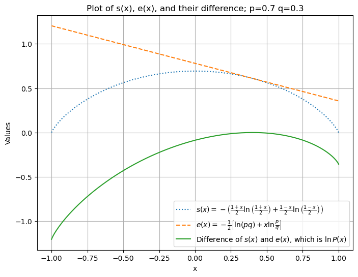
Notice:
\(s(x)\) and \(e(x)\) are the entropy and energy per coin, respectively (see legend).
The entropy \(s(x)\) has a maximum at the neutral point \(x = 0\) and vanishes at the boundaries (all spin up / down)/
“Low energy” states have higher probability.
The competition between \(e(x)\) and \(s(x)\) leads to a maximum in their difference, \(s(x)-e(x)\).
Later, we will rather look at the negative, \(e(x)-s(x)=:f(x)\), which we call a free energy. It is generally a convex function and has a minimum at the most likely value of \(x\).
Note
The depicted maximum in \(-f(x)\) does not look very impressive. But, since we have
a so-called (large deviation principle)[https://en.wikipedia.org/wiki/Large_deviations_theory], we will get a pronounced maximum at \(x=p-q\) (the minimum of \(f(x)\)) for even modestly large \(N\). Fully deterministic behavior \(x \to p-q\) emerges in the thermodynamic limit, \(N\to \infty\). The most likely value of \(x\) coincides with the expectation value \(\langle x \rangle = p-q\) (see below).
We can explore the effects of finite \(N\) by Taylor expanding \(S(x)-E(x)\) to \(O(\Delta x^2)\equiv O\left[(x-\langle x\rangle)^{2}\right]\), we obtain to leading order a Gaussian,
whose spread is controlled by the variance \(\langle \Delta x^2\rangle = 4pq N^{-1/2}\).
Note
One can show that, quite generally, large sums of random variables tend to Gaussians if correlations are short ranged. This is a consequence of the Central Limit Theorem (CLT). The Gaussian is completely fixed by knowing the first and second moment of the distribution. Since the first two moments can often be determined quite easily (see below), this is a great advantage for calculations. The scaling \(\langle \Delta x^2\rangle\sim N^{-1/2}\) and the fact that the limiting distribution is independent of the higher order details of the distributions of individual random numbers is a first example of universality. See Section 1.5 of Arovas for a clear mathematical demonstration of the CLT.
Calculation of first and second moment#
The \(n^\text{th}\) moment of a random variable X is defined by \(\langle X^n\rangle\). The first and second moment of a distribution can often be computed analytically, and those are needed in the context of the CLT. Higher order moments are often more challenging to obtain.
Expectation value#
So, we see that the expectation value of X is an extensive quantity.
Of course, a particular realization will (usually!) not have \(X=\langle X\rangle\).
One measure of spread is the
Variance#
To compute \(\left\langle X^{2} \right\rangle\):
if \(i=j: \sigma_{i} \cdot \sigma_{i}=1 \text {, so }\left\langle\sigma_{i} \cdot \sigma_{i}\right\rangle=1\)
if \(j\neq j: \left\langle\sigma_{i} \sigma_{j}\right\rangle=\left\langle\sigma_{i}\right\rangle\left\langle\sigma_{i}\right\rangle=(p-q)^{2}\)
So, \(\left\langle X^{2}\right\rangle=N+N(N-1)(p-q)^{2}\) v. \(\langle X\rangle^{2}=N^{2}(p-q)^{2}\)
Note: Since \(\Delta X \propto \sqrt{N}\) but \(\langle X\rangle\propto N\), we have \(\frac{\Delta x}{\langle x\rangle} \sim N^{-1/2}\rightarrow 0\) for \(p \neq q\) as \(N\to \infty\).
The \(\sqrt{N}\) scaling is a general consequence of the CLT.
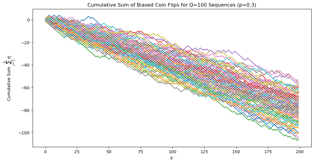
Simulating coin-flips as random walks#
# Parameters
S = 10000 # Number of samples (sequences)
N = 200 # Length of each sequence
Q = 100 # Number of sequences to plot
# Parameters for the biased coin
p = 0.3 # Probability of getting +1 (heads)
q = 1 - p # Probability of getting -1 (tails)
# Generate S samples of N biased coin flips
biased_coin_flips = np.random.choice([1, -1], (S, N), p=[p, q])
# Plot 1: Sum of sigma_j from j=1 to k for Q of the S sequences (with biased coin)
plt.figure(figsize=(12, 6))
for i in range(Q):
plt.plot(np.cumsum(biased_coin_flips[i, :]), label=f'Sequence {i+1}')
plt.xlabel(r'$k$')
plt.ylabel(r'Cumulative Sum $\sum_{j=1}^k \sigma_j$') #'Cumulative Sum of Sigma_j'
plt.title(f'Cumulative Sum of Biased Coin Flips for Q={Q} Sequences (p={p})')
plt.show()
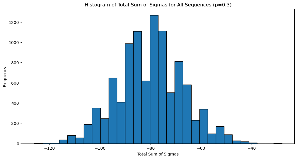
# Plot 2: Histogram of the total sum of the sigmas of all sequences (with biased coin)
biased_total_sums = np.sum(biased_coin_flips, axis=1)
plt.figure(figsize=(12, 6))
plt.hist(biased_total_sums, bins=30, edgecolor='black')
plt.xlabel('Total Sum of Sigmas')
plt.ylabel('Frequency')
plt.title(f'Histogram of Total Sum of Sigmas for All Sequences (p={p})')
plt.show()
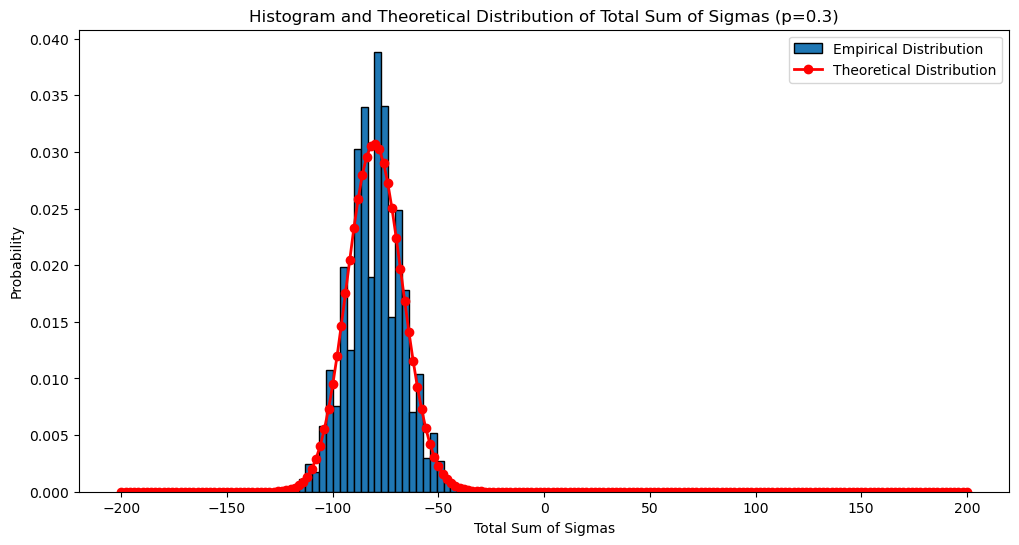
from scipy.stats import binom

# Theoretical expectation for the probability distribution of the sum of sigmas
# The sum of S sigmas is equivalent to the number of heads minus the number of tails.
# This can be modeled by a binomial distribution, where 'success' is getting a head (+1).
# The total sum can range from -N (all tails) to +N (all heads).
# The probability of k heads is binom.pmf(k, N, p), where k ranges from 0 to N.

# Adjusting k to represent the sum of sigmas: k heads and N-k tails gives a sum of 2k-N.
# The theoretical probabilities need to be scaled accordingly.
theoretical_probs = [binom.pmf(k, N, p)/2 for k in range(N + 1)]
scaled_sums = np.array([2 * k - N for k in range(N + 1)])

# Plotting the histogram with the theoretical distribution
plt.figure(figsize=(12, 6))
plt.hist(biased_total_sums, bins=30, edgecolor='black', density=True, label='Empirical Distribution')
plt.plot(scaled_sums, theoretical_probs, color='red', marker='o', linestyle='-', linewidth=2, label='Theoretical Distribution')
plt.xlabel('Total Sum of Sigmas')
plt.ylabel('Probability')
plt.title(f'Histogram and Theoretical Distribution of Total Sum of Sigmas (p={p})')
plt.legend()
plt.show()