When does quantum mechanics make a difference?

Following Kardar 6.1 and 6.2, we’ll motivate quantum statistical mechanics with some cases where classical mechanics gives incorrect answers or even diverges, before developing the general formalism.

Fluctuations of a Hydrogen atom

Consider the classical Hamiltonian for a hydrogen atom:

\[ H = \frac{p_{1}^{2}}{2 m_{e}} + \frac{p_{2}^{2}}{2 m_{p}} + V\left(r_{1} - r_{2}\right) \]

Determine the partition function \(Z(T)\), the free energy \(F(T)\), the internal energy \(E(T)\), and other thermodynamic quantities.

We begin by transforming to center of mass and relative coordinates. Define the center of mass coordinates as \(\vec{R} = \frac{1}{M}(m_e \vec{r}_1 + m_p \vec{r}_2)\) with total momentum \(\vec{P}\), and the relative coordinates as \(\vec{r} = \vec{r}_1 - \vec{r}_2\) with relative momentum \(\vec{p}\). The Hamiltonian then separates into:

\[ H = \frac{P^2}{2M} + \frac{p^2}{2\mu} + V(\vec{r})\;, \]

where \(M = m_e + m_p\) is the total mass, and \(\mu = \frac{m_e m_p}{m_e + m_p}\) is the reduced mass.

The center of mass and relative motions separate, allowing the partition function to factorize as \(Z = Z_{\mathrm{cm}} \cdot Z_{r}\). For the relative motion, the partition function is given by:

(26)\[\begin{split} \begin{aligned} Z_{r} & = \int \frac{d^{3}p \, d^{3}r}{h^{3}} \, e^{-\beta \left(\frac{p^{2}}{2\mu} + V(r)\right)} \\ & = \frac{1}{\lambda_\mu^{3}} \cdot 4\pi \int_{0}^{\infty} dr \, r^{2} \, e^{+\beta \frac{e^{2}}{4\pi\epsilon_{0}r}} \end{aligned} \end{split}\]

where the thermal de Broglie wavelength is defined as:

\[ \lambda_\mu \equiv \sqrt{\frac{h^2 \beta}{2\pi \mu}}. \]

At short wavelengths, classical mechanics encounters a problem. The integral in Eq.~(26) diverges because \(e^{r_{0} / r} \rightarrow \infty\) as \(r \rightarrow 0\)

Quantum mechanics addresses this problem through Heisenberg’s uncertainty principle:

\[ \Delta p \Delta r \geq h \]

This principle leads to a discrete set of energy levels:

\[ \hat{H}\left|E_{\alpha}\right\rangle = E_{\alpha}\left|E_{\alpha}\right\rangle \]

Rather than using the classical partition function:

\[ Z = \int \frac{d q \, d p}{h} e^{-\beta H(q, p)}, \]

we adopt the quantum mechanical formulation:

(27)\[ \boxed{Z = \sum_{\alpha} e^{-\beta E_{\alpha}}} \]

This quantum partition function is well-defined and avoids the divergences inherent in the classical approach. The examples below demonstrate how this quantum formulation transitions to classical results in the high-temperature limit (\(T \rightarrow \infty\)).

In approximately two lectures, we will derive (27) from a more formal perspective on quantum statistical mechanics.

It is important to note that in (27), the summation is over all measurable quantum states \(\alpha\), which serve as the quantum analog of microstates in classical statistical mechanics.

Dilute Polyatomic Gases

Let’s consider a gas composed of tightly bound molecules. For each molecule, the internal Hamiltonian is given by

\[ H=\sum_{i=1}^{n} \frac{p_{i}^{2}}{2 m}+V\left(q_{1}, \cdots, q_{n}\right), \]

where \(n\) is the number of atoms per molecule. We’ve rescaled variables so that all particles have the same effective mass \(m\) by transforming \(q_i \rightarrow q_i \sqrt{m_i/m}\) and \(p_i \rightarrow p_i \sqrt{m/m_i}\), preserving the phase space volume element \(dq \cdot dp\).

The partition function for a single molecule is:

\[ Z_1 = \int \prod_{i=1}^{n} \frac{d^3 q_i d^3 p_i}{h^3} , e^{-\beta\left(H_{\text{kin}} + V(\vec{q})\right)}. \]

For \(N\) such molecules (neglecting interactions), the total partition function is:

\[ Z(N) = \frac{Z_1^N}{N!}. \]

(Note: there’s no factor of \(1/n!\) unless the atoms are identical.)

The interaction potential \(V\) has a typical energy scale on the order of the Rydberg:

\[ R_y \sim 13.6,\text{eV} \approx 1160\text{K} \cdot k_B. \]

For temperatures \(T < 1000,\text{K}\), the molecules remain tightly bound and fluctuate around a stable equilibrium configuration \(q_i^*\). Defining \(u_i = q_i - q_i^*\) and expanding to second order:

\[ V({q_i}) \approx V^* + \frac{1}{2} \sum_{i,j} \frac{\partial^2 V}{\partial q_i \partial q_j} u_i \cdot u_j, \]

where \(V^* = V({q_i^*})\) and the first derivatives vanish at equilibrium. The Hessian matrix is symmetric and positive definite and can be diagonalized:

\[ \frac{\partial^2 V}{\partial q \partial q} = O^\top K O, \quad K = \text{diag}(K_s), \]

with \(O\) orthogonal. Defining transformed variables:

\[ \tilde{u} = O u, \quad \tilde{p} = O p, \]

the partition function becomes:

\[ Z = \int \prod_{i=1}^n \frac{d^3 \tilde{u}_i d^3 \tilde{p}_i}{h^3} e^{-\beta\left(\frac{1}{2m} \tilde{p}^\top \tilde{p} + V^* + \frac{1}{2} \tilde{u}^\top K \tilde{u}\right)}. \]

This separates into kinetic and potential parts. Using:

\[ \lambda = \sqrt{\frac{h^2 \beta}{2\pi m}}, \]

and integrating over all \(\tilde{p}_i\), we get:

\[ Z = \frac{1}{\lambda^{3n}} \prod_{s=1}^{3n} \int d\tilde{u}_s e^{-\beta \frac{K_s}{2} \tilde{u}_s^2} = \prod_{s=1}^{3n} \sqrt{\frac{m}{K_s h^2 \beta^2}}. \]

The internal energy follows as:

\[ E = -\partial_\beta \ln Z = 3n k_B T, \]

which reflects the classical equipartition result: \(\frac{1}{2}k_B T\) per quadratic degree of freedom.

If any \(K_s = 0\), that mode contributes no \(\beta\)-dependence, and hence no contribution to \(E\). Let \(m\) be the number of nonzero modes, then:

\[ E = \frac{3n + m}{2} k_B T. \]

The number of zero modes \(r = 3n - m\) is determined by symmetry—typically 3 translational and 0–3 rotational modes, depending on whether the molecule is mono-, di-, or polyatomic.

Therefore, the heat capacity per molecule is:

\[ C_v = \left.\frac{dE}{dT}\right|_V = \left(3n - \frac{r}{2}\right) k_B. \]

This predicts a temperature-independent \(C_v\).

However, this is not what is observed in experiments: at low temperatures, many degrees of freedom are “frozen out” due to energy quantization, and \(C_v\) increases stepwise with temperature as different modes become accessible.

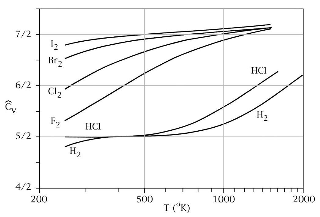
For \(H_{2}\), a diatomic molecule, we have \(n=2\) and \(r=5\), accounting for 3 translational and 2 rotational degrees of freedom.

The predicted heat capacity is:

\[ \frac{C_V}{k_B} = 6 - \frac{5}{2} = \frac{7}{2} = \frac{\text{3 translational + 2 rotational + 1 vibrational}}{2}. \]

However, the observed behavior varies with temperature:

• As \(T \rightarrow 0\), \(C_V \sim \frac{3}{2} k_B\) due to center-of-mass translation.

• Around \(T \sim 500 \, \mathrm{K}\), \(C_V \sim \frac{5}{2} k_B\), reflecting contributions from center-of-mass translation and rotation.

• At \(T \gg 1000 \, \mathrm{K}\), \(C_V \sim \frac{7}{2} k_B\), including contributions from center-of-mass translation, rotation, and vibration.

Classical results are only recovered when \(k_B T > \mathrm{eV}\). At intermediate temperatures, certain degrees of freedom remain “frozen out” due to energy quantization effects.

Vibrational Modes

A diatomic molecule has \(3 \cdot 2 - 5 = 1\) vibrational mode with \(K_s > 0\), corresponding to the oscillation of the bond connecting the two atoms.

Let \(q = x - x_0\) represent the bond length deviation from its equilibrium value \(x_0\). The vibrational Hamiltonian is given by:

\[ H_{\text{vib}} = \frac{p^2}{2m} + \frac{K_s q^2}{2} = \frac{p^2}{2m} + \frac{m \omega^2}{2} q^2, \]

where \(\omega = \sqrt{K_s / m}\) is the classical vibrational frequency.

Classically, the partition function is:

\[ Z = \frac{1}{\lambda} \sqrt{\frac{2\pi}{\beta K_s}} = \sqrt{\frac{m}{K_s \hbar^2 \beta^2}} = \frac{k_B T}{\hbar \omega} = \frac{1}{\beta \hbar \omega}. \]

The corresponding internal energy is:

\[ E = \langle H \rangle = -\partial_\beta \ln(Z) = k_B T, \]

which reflects two degrees of freedom.

In quantum mechanics, the energy eigenstates are given by:

\[ \hat{H}|n\rangle = \hbar \omega \left(n + \frac{1}{2}\right)|n\rangle, \quad n = 0, 1, 2, \dots \]

The partition function can be computed as:

\[ \begin{aligned} Z & = \sum_{n= & =\frac{e^{-\beta \hbar \omega / 2}}{1-e^{-\beta \hbar \omega}}=\frac{1}{2 \sinh (\beta \hbar \omega / 2)} \end{aligned} \]

\[ Z=\frac{e^{-\beta \hbar \omega / 2}}{1-e^{-\beta \hbar \omega}}=\frac{1}{2 \sinh (\beta \hbar \omega / 2)} \]

As \(\quad T \rightarrow \infty\), \(\beta \rightarrow 0\), we get the classical result,

\[ \lim _{T \rightarrow \infty} Z=\frac{1}{\beta\hbar\omega}=Z_{\text {classical }} \]

Note this required the \(\int \frac{d q d p}{h}\) we’ve conventionally put in the classical phase-space integral. While it doesn’t affect observables, it arises from the semiclassical principle!

Note

Quantum states and phase space volume

Each quantum state occupies a phase space volume of \(2 \pi \hbar\). This relationship arises from the Bohr-Sommerfeld quantization condition:

\[ S = \int_{\partial S} p(q) \cdot dq = n \cdot h, \]

where \(S\) represents the action, and \(n\) is an integer.

The phase space volume can also be expressed as:

\[ \int_{\partial S} p \, dq = \int_{S} dp \wedge dq, \]

which corresponds to the total phase space volume enclosed. This principle is foundational to the Weyl formula and the Gutzwiller trace formula.

Since \(\ln (Z) = \ln (2) - \ln (\sinh (\beta \hbar \omega / 2))\), the internal energy is given by:

\[ E = -\partial_\beta \ln Z = \frac{\hbar \omega}{2} \coth \left(\frac{\beta \hbar \omega}{2}\right) = \frac{\hbar \omega}{2} \frac{e^{\beta \hbar \omega} + 1}{e^{\beta \hbar \omega} - 1}. \]

To visualize this function, we plot the reduced energy \(\frac{E}{\hbar \omega}\) as a function of the reduced temperature \(T / \theta_\text{vib}\), where \(\theta_\text{vib} = \frac{\hbar \omega}{k_B}\) is the vibrational temperature.

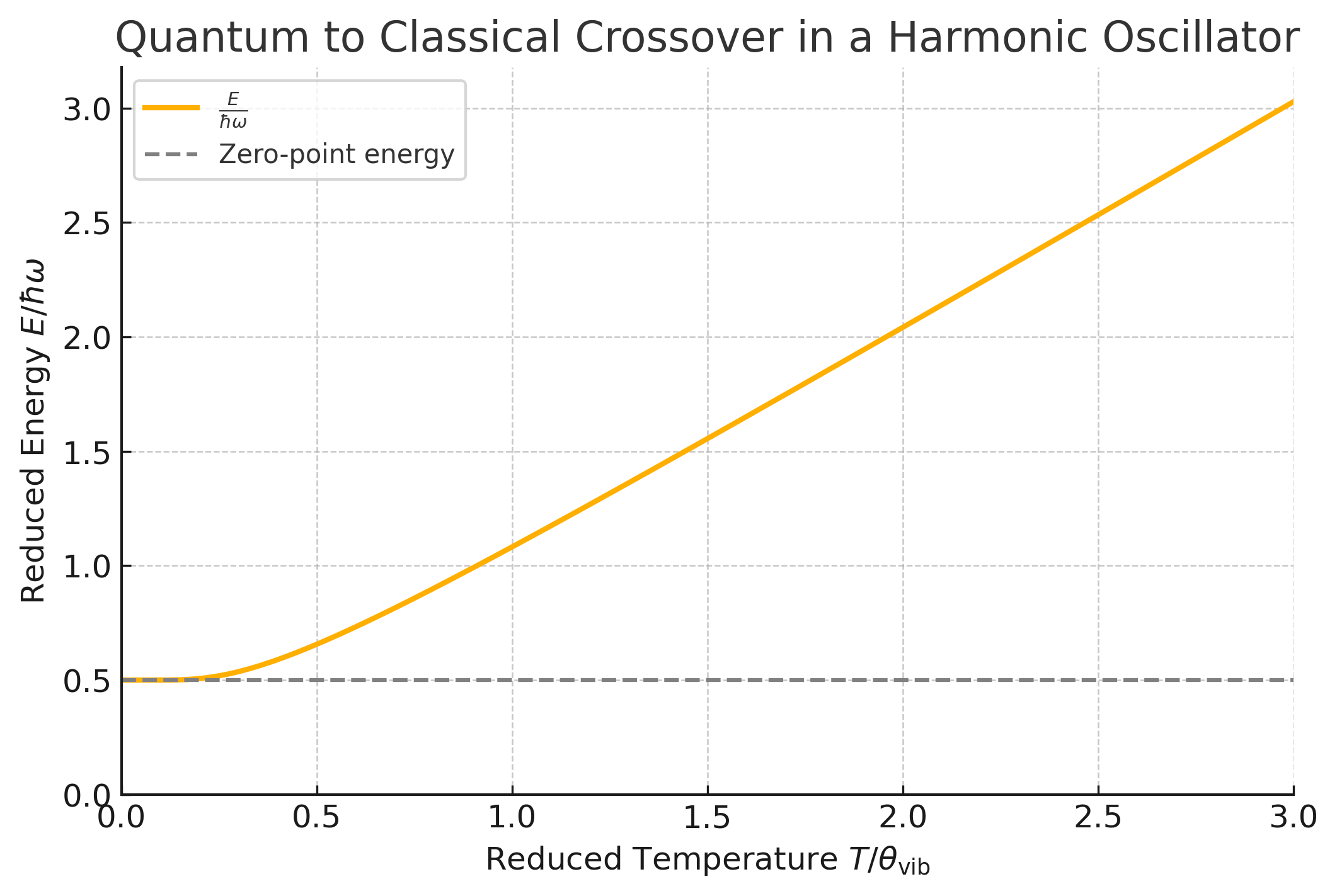
Fig. 1 Plot of the reduced energy \(\frac{E}{\hbar \omega}\) as a function of the reduced temperature \(T / \theta_\text{vib}\). The energy approaches \(\frac{1}{2}\) at low temperatures and increases linearly with \(T / \theta_\text{vib}\) at high temperatures, reflecting the transition from quantum to classical behavior.

The plot shows that at low temperatures (\(T / \theta_\text{vib} \ll 1\)), the energy approaches the zero-point energy \(\frac{\hbar \omega}{2}\). At high temperatures (\(T / \theta_\text{vib} \gg 1\)), the energy asymptotically approaches the classical result \(k_B T\).

\[ C_V=\partial_T E=k_{B}\left(\frac{k \omega}{k_{B} T}\right)^{2} \frac{e^{-\beta \hbar \omega}}{\left(1-e^{-\beta A \omega}\right)^{2}} \]

Note

Note \(\frac{C_V}{K_{B}} \sim\left(\frac{\hbar w}{K_{B} T}\right)^{2} e^{-\hbar \omega / K_{B} T}\) is exponentially small as \(T \rightarrow 0\). This is a general feature of any model with a gap \(\Delta E=\hbar \omega \) above ground state.

Rotations

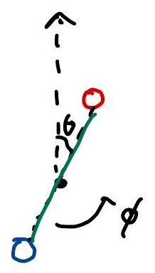
The orientation of a diatomic molecule can be described using the angles \(\theta\) and \(\varphi\), which parameterize a point on the surface of a 3D ball (\(S_2\)). The Lagrangian for the system is:

\[ L = \frac{I}{2} \left(\dot{\theta}^2 + \sin^2 \theta \, \dot{\phi}^2\right), \]

where \(I\) is the moment of inertia. The conjugate momenta are given by:

\[ p_{\theta} = \frac{\partial L}{\partial \dot{\theta}} = I \dot{\theta}, \quad \rho_{\phi} = \frac{\partial L}{\partial \dot{\phi}} = I \sin^2 \theta \, \dot{\phi}. \]

The Hamiltonian, expressed in terms of these momenta, is:

\[ H = p \dot{q} - L = \frac{1}{2I} \left(\rho_{\theta}^2 + \frac{\rho_{\phi}^2}{\sin^2 \theta}\right) = \frac{\vec{L}^2}{2I}, \]

where \(\vec{L}\) is the angular momentum vector. This formulation is analogous to the dynamics of a particle constrained to move on the surface of a unit ball.

Classically, the partition function is given by:

\[\begin{split} \begin{aligned} Z & = \frac{1}{h^{2}} \int_{0}^{\pi} \int_{0}^{2 \pi} d\theta \, d\phi \int d\rho_{\theta} \, d\rho_{\phi} \, e^{-\frac{\beta}{2I} \left(\rho_{\theta}^{2} + \frac{\rho_{\phi}^{2}}{\sin^{2} \theta}\right)} \\ & = \frac{1}{h^{2}} \int_{0}^{\pi} \int_{0}^{2 \pi} d\theta \, d\phi \, \sqrt{\frac{2 \pi I}{\beta}} \sqrt{\frac{2 \pi I \sin^{2} \theta}{\beta}} \\ & = \frac{2 \pi I}{\beta h^{2}} \int_{0}^{\pi} d\theta \, \sin \theta \int_{0}^{2 \pi} d\phi \\ & = \frac{2 \pi I}{\beta} \cdot \frac{4 \pi}{h^{2}}. \end{aligned} \end{split}\]

From this, we find:

\[ \ln(Z) \propto -\ln(\beta), \]

which implies the energy and heat capacity are:

\[ E = k_B T, \quad C_V = k_B. \]

This result corresponds to two degrees of freedom, associated with \(\rho_{\theta}\) and \(\rho_{\phi}\).

Quantum mechanically, the rotational Hamiltonian is expressed as:

\[ H = \frac{\vec{L}^2}{2I}, \]

where \(\vec{L}\) is the angular momentum operator. However, the components of \(\vec{L}\) do not commute:

\[ \left[L_i, L_j\right] \neq 0. \]

The wavefunctions are spherical harmonics, \(\psi(\theta, \phi) = Y_{l, m}(\theta, \phi)\), with eigenvalues:

\[ \vec{L}^2 = \hbar^2 l(l+1), \quad -l \leq m \leq l. \]

The quantum partition function is given by:

\[\begin{split} \begin{aligned} Z_1 & = \sum_{l=0}^\infty \sum_{|m| \leq l} e^{-\frac{\beta}{2I} \hbar^2 l(l+1)} \\ & = \sum_{l=0}^\infty (2l + 1) e^{-\frac{\beta}{2I} \hbar^2 l(l+1)}. \end{aligned} \end{split}\]

In the high-temperature limit (\(T \to \infty\), \(\beta \to 0\)), the summation over \(l\) can be approximated by an integral:

\[ \lim_{T \to \infty} Z = \frac{T}{\theta_r}, \quad \theta_r = \frac{h^2}{2I k_B}, \]

recovering the classical result \(Z_{cl}\).

At low temperatures (\(T \to 0\)), the partition function simplifies to:

\[ Z = 1 + 3 e^{-2\theta_r / T}, \]

leading to a steep drop in the specific heat as \(T \to 0\). The rotational energy is approximately:

\[ E_{rot} = -\partial_\beta \ln(Z) \approx 6k_B \theta_r e^{-2\theta_r / T}, \]

and the specific heat is:

\[ C_{rot} = \partial_T E_{rot} \approx 3k_B \left(\frac{2\theta_r}{T}\right)^2 e^{-2\theta_r / T}. \]

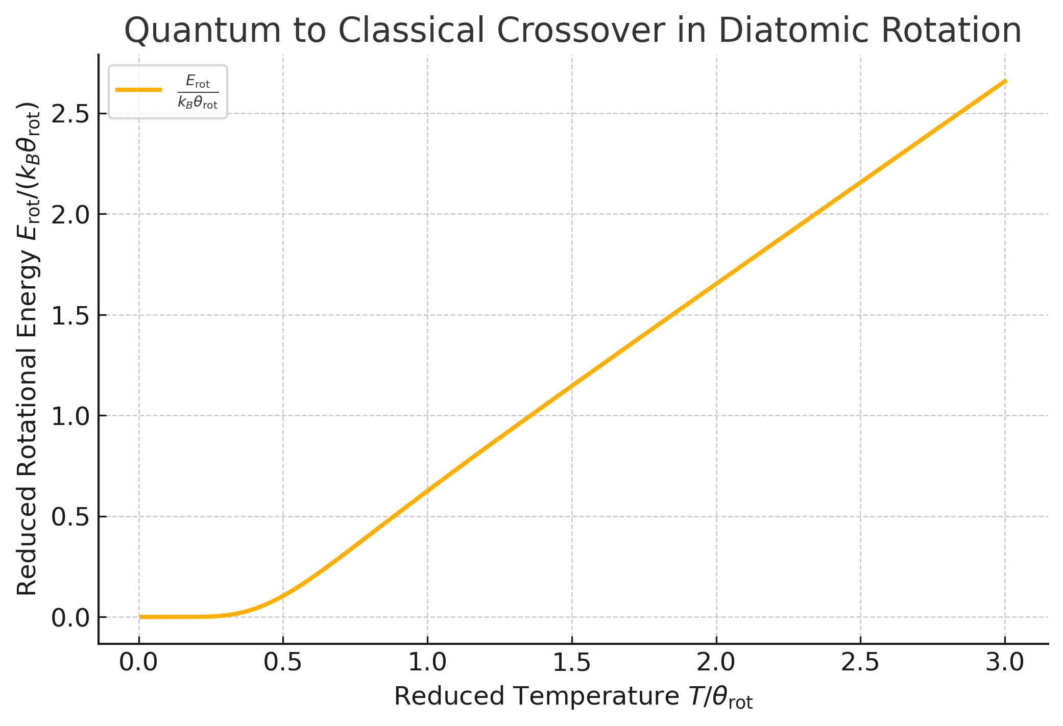
Fig. 2 Plot of the reduced rotational energy \(E_{rot} / k_B \theta_r\) as a function of the reduced temperature \(T / \theta_r\). The energy approaches zero at low temperatures due to quantum effects and increases linearly with \(T / \theta_r\) at high temperatures, reflecting the transition to classical behavior.

Note

Why is there no zero-point rotational energy?

In quantum mechanics, zero-point energy arises when a system is confined by a potential, such as in a harmonic oscillator. The uncertainty principle prevents the particle from being completely at rest, leading to a nonzero ground-state energy:

\[ E_0^{\text{vib}} = \frac{1}{2} \hbar \omega \]

In contrast, for a rigid rotor (like a diatomic molecule), the system moves freely on a sphere without a confining potential. Its energy levels are:

\[ E_\ell = \frac{\hbar^2}{2I} \ell(\ell + 1), \quad \ell = 0, 1, 2, \dots \]

The ground state (\(\ell = 0\)) has:

\[ E_0^{\text{rot}} = 0 \]

Since there’s no restoring force and no potential minimum, there’s no quantum requirement for zero-point rotational motion.