Brownian Motion as a Free Energy Minimizing Process

Brownian Motion as a Free Energy Minimizing Process#

Consider a suspension of a large number of ideal beads:

Goal:#

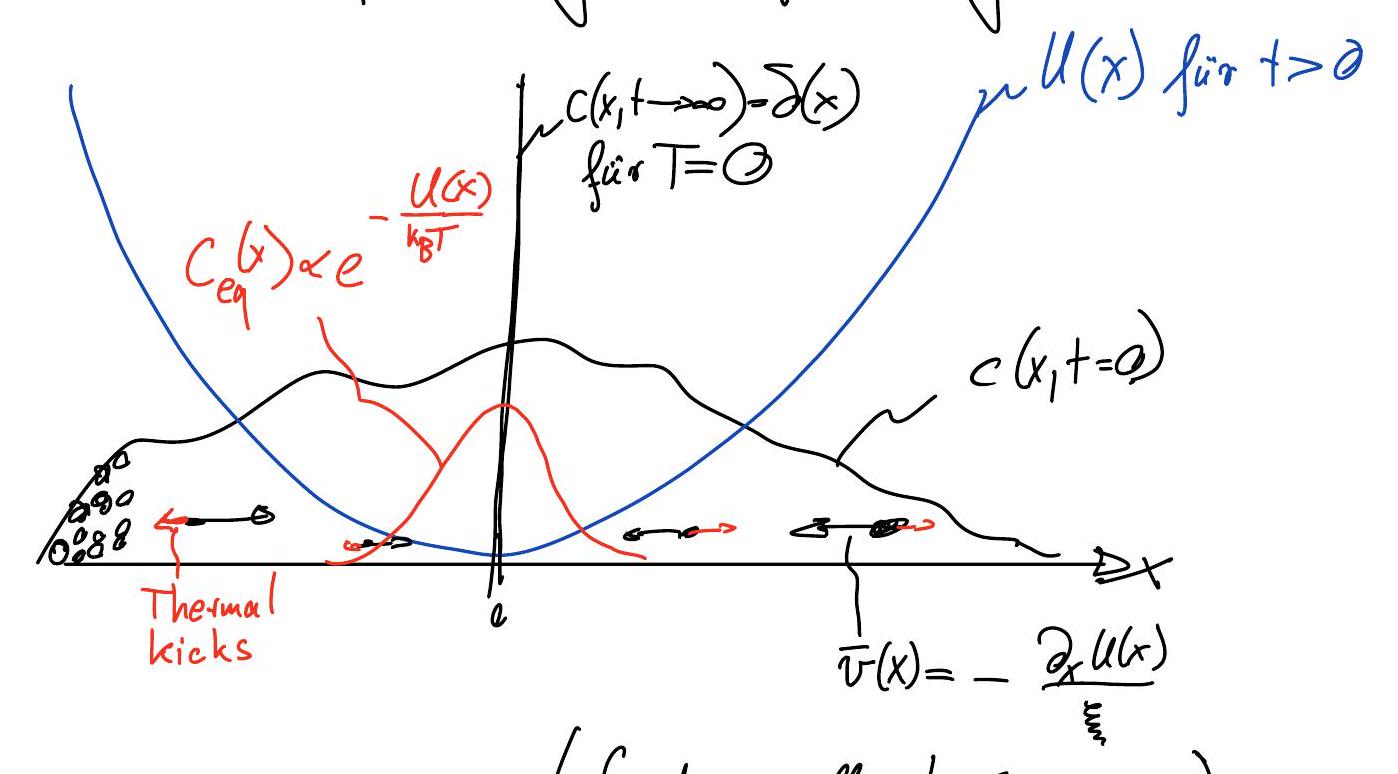
Construct a phenomenological model for the dynamics of the particle density $c(x, t)$ at position $x$ and time $t$ that leads to the equilibrium (Boltzmann) distribution

\[ c(x, t) \longrightarrow c_{eq}(x) \sim e^{-\frac{U(x)}{k_B T}}. \]

Based on simple and natural assumptions, we will be led to the generalized diffusion equation. One nice (and strange) feature of these dynamics is that they continuously lower the free energy.

Conservation of Particle Number#

The conservation of particle number requires that the dynamical equation of motion is described by the continuity equation:

\[ \frac{\partial c(x,t)}{\partial t} = -\frac{\partial j(x,t)}{\partial x} \tag{1} \]

where $j(x,t)$ is the probability current, i.e., the number of particles crossing $x$ per unit time.

The probability current $j(x, t)$ has two contributions:#

Deterministic motion (drift due to potential $U(x)$):

\[ j_{\text{det}} = c \cdot \bar{v} = -\frac{c}{\xi} \frac{\partial U}{\partial x} \]

where we introduced the mean velocity $\bar{v}=-\partial_x U/\xi$ of an overdamped particle in a potential $U$. The friction coefficient $\xi$ for a spherical particle of diameter $\sigma$ in a fluid of viscosity $\eta$ is given by:

\[ \xi = 6 \pi \eta \sigma \]
Random motion (diffusion):

\[ j_{\text{diff}} = -D \frac{\partial c}{\partial x} \quad \text{(Fick’s Law)} \]

Total current:#

Combining both contributions yields

\[ j = j_{\text{det}} + j_{\text{diff}} \;, \]

which can be rewritten as $j=c v_{fl}$ in terms of a net velocity $v_{fl}$,

\[ v_{fl} = -\xi^{-1} \frac{\partial}{\partial x} \left( U + D \xi \ln c \right) = -\xi^{-1} \frac{\partial \mu}{\partial x} \;, \]

where $\tilde \mu(x)$ is defined as $$ \tilde \mu(x) = D \xi \ln c + U(x);. $$

Note that $\tilde \mu(x)$ is the local chemical potential for non-interacting particles if we could replace $D\xi$ by $k_B T$. We will soon see that this has to be the case to reproduce the Bolzmann distribution in equilibrium.

Generalized Diffusion Equation#

Substituting this into the continuity equation gives

\[ \frac{\partial c}{\partial t} = -\partial_x j =\frac{\partial}{\partial x}\left( \frac{c}{\xi} \frac{\partial \tilde \mu}{\partial x} \right) = \frac{\partial}{\partial x} \left( \frac{1}{\xi} \left( D \xi \frac{\partial c}{\partial x} + c \frac{\partial U}{\partial x} \right) \right). \]

Equilibrium ($t \to \infty$):#

At equilibrium, $\frac{\partial c}{\partial t} = 0$ implies $j=0$, so:

\[ \tilde \mu = U + D \xi \ln c_{eq} = \text{const}. \]

Solving for $c_{eq}$:

\[ c_{eq} \propto \exp \left( -\frac{U(x)}{D \xi} \right). \]

Since this must reproduce the Boltzmann distribution:

\[ c_{eq} \propto \exp \left( -\frac{U(x)}{k_B T} \right), \]

we require the Stokes-Einstein relation:

\[ D=\frac{k_B T}{\xi}. \]

This is a key example of a fluctuation-dissipation theorem. So, indeed, $\tilde \mu= \mu$, the local chemical potential.

Example values:#

For a spherical particle with radius $R$: $\xi = 6 \pi \eta R$.
Proteins ($R \approx 2$ nm): $D \approx 100 \, \mu m^2/s$.
Bacteria: $D_{bac} \approx 0.5 \, \mu m^2/s$.

(For physical intuition, it’s helpful to anticipate $ \langle \Delta x^2 (t) \rangle = 2 D t$.)

Generalization: Multiple degrees of freedom#

Knowing $\mu=$const. in equilibrium suggests that, close to equilibrium, gradients of the chemical potential should act as driving forces towards equilibrium. This insight can be used to construct Brownian motion for a complex system with potentially very many degrees of freedom $\{x_i\}$. Here, $x_i$ could be the position of a segments of a polymer or a membrane, or just coordinates of interacting particles. The gradient $F_i=-\partial_i \mu$ is the thermodynamic driving force.

As before, we demand a continuity equation,

\[ \partial_t \Psi(\{x_i\}_i) = -\sum_i \partial_i j_i, \]

where $j_i = \Psi v_i$ and

\[ v_i = \sum_j H_{ij} F_j \]

with mobility matrix $H_{ij}$ and forces:

\[ F_j = -\partial_j \mu, \quad \mu = U + k_B T \ln \Psi. \]

This is known as the Smoluchowski equation.

Free Energy Minimization#

Define the free energy functional:

\[ F[c] = \int dx \, c(x, t) \mu(x). \]

The free energy is monotonically decreasing under Brownian motion:

\[ \frac{dF}{dt} = \int dx \left[ \mu \frac{\partial c}{\partial t} + c \frac{\partial \mu}{\partial t} \right]. \]

Using integration by parts and boundary conditions at infinity, we obtain:

\[ \frac{dF}{dt} = -\int dx \left[ c (\partial_x\mu)^2 + k_B T \partial_t c \right] \;, \]

which is negative unless $\mu=$const., i.e., we have reached equilibrium.

Note: The dynamics are time-irreversible due to coarse-graining and underlying microscopic chaos (see next lecture on ergodicity).

Diffusion Equation – Basic Solution:#

For $U = 0$:

\[ \frac{\partial c(x, t)}{\partial t} = D \partial_{x}^{2} c(x, t) \tag{2} \]

Diffusion

Assume $c(x,0) = \delta(x)$ (point source at $x=0$).

Fourier transform of (2):

\[ c(x, t)=\int_{-\infty}^{\infty} \frac{d q}{2 \pi} e^{-i q x} c(q, t), \quad \frac{\partial c(q, t)}{\partial t} = -D q^{2} c(q, t). \]

Solution:

\[ c(q, t) = e^{-D q^{2} t}. \]

Inverse Fourier transform:

\[ c(x, t) = \frac{e^{-x^{2}/(4 D t)}}{\sqrt{4 \pi D t}} = \frac{e^{-x^{2}/(2 \sigma_t^{2})}}{\sqrt{2 \pi \sigma_t^{2}}} \]

with $\sigma_t^2 = 2 D t$.

Note: This is the Green’s function solution. For arbitrary initial conditions, convolve with this Green’s function.

Since particles are non-interacting:

\[ c(x, t) = N \cdot p(x, t), \]

where $p(x, t)$ is the probability density for a single particle.

Practical Example: Nerve Cell Transport#

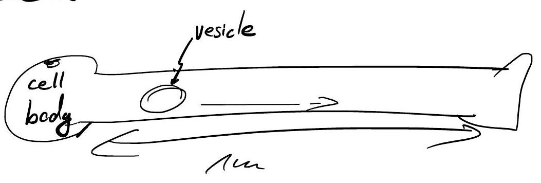
Is diffusion fast enough to transport vesicles?

Given $D \approx 0.5 \, \mu m^2/s$:

\[ \frac{\langle x^2 \rangle}{2 D} \approx 12 \, \text{days!} \]

$\Rightarrow$ Nerve cells require active transport (e.g., via motor proteins).

Example: Bacteria#

For $L \approx 1 \, \mu$m and $D \approx 100 \, \mu m^2/s$:

\[ t \approx \frac{L^2}{2D} \approx 2 \, \text{ms}, \]

which is much shorter than the $20$ min lifecycle of E. coli $\rightarrow$ diffusion is effective for bacteria.

Application: Diffusion-limited Reaction Rates#

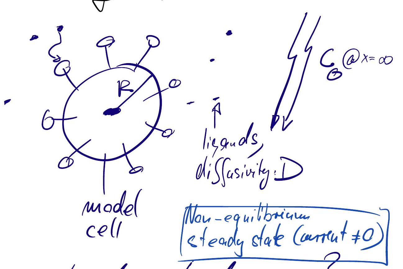
Ligand capture rate:#

How many ligands are captured per sec?

Use diffusion equation to model the ligands: $$ \partial_{t} c=D \nabla^{2} c=D\left(\partial_{x}^{2} c+\partial_{y}^{2} c+\partial_{z}^{2} c\right) $$

\[ \partial_{t} c=D \frac{1}{r^{2}} \partial_{r}\left(r^{2} \partial_{r} c\right) ; c=c\left(r, t\right) \]

Steady state: $0=\partial_{t} c_s$, so, $ \partial_{r} c_{s}=\frac{\text { const }}{r^{2}}$ for $r>R$

\[ c_{s}(r)=\frac{-A}{r}+B=-\frac{A}{r}+c_{0} \Rightarrow c_{s}(\infty)=c_0 \]

Perfect absorber limit: $c_{s}(R)=0$.

\[ \Rightarrow c_{s}(r)=c_{0}\left(1-\frac{R}{r}\right) . \]

The particle current is $j(R)=|\vec{j}(\vec{R})|=D \partial_{r} c(r, t)=\frac{D c_0 R}{R^{2}}$.

Thus, the total flux of captured ligands is given by the expression

\[ \Phi = j(R) 4\pi R^2=4\pi D c_0 R \]

(Check dimensions!)

Universal Bound on Reaction Rates#

Key question: How fast is $A+B \xrightarrow{k} C$ if it is limited by $A-B$ collision rates?

In the extreme case, where each A-B collision leads to a C particle we have $k=c_{A}\tilde{k}_{A-B}$, where where $\tilde{k}_{A-B}$ is the rate of which a focal A particle is hit by B particles.

Since $x_{A}-x_{B}$ diffuses w/ twice the diffusion constant, we have that the number of collisions per unit time of B particles with a focal A particle is given by the above rate of ligand capture with twice the diffusivity and with twice the radius,

\[ \tilde{k}_{A-B}=4 \pi(2 D)(2 R) C_{B} \]

\[ \Rightarrow \frac{\partial C_{C}}{\partial t}=k_{\text {diff }} C_{A} \cdot C_{B} \]

where

\[ \begin{gathered}k_{\text {diff }}=16 \pi D R=16 \pi R \frac{k_{B} T}{6 \pi n R}=\frac{8 k_{B} T}{3 \eta} \end{gathered} \]

for spherical particles. Note that this is a nice universal bound, dependent only on temperature and viscosity. For water at room temperature, one estimates

\[ k_{\text {diff }}\approx 7 \cdot 10^9 \frac{1}{M \cdot s} \]

Notes:

Most enzymes are 100-1000 times slower $\Rightarrow$ they require more than just one collision to form a product.
… could be modeled by assuming a finite absorption rate.
Relation to Michaelis-Menten kinetics: Rate of product formation =$k_{max}[E][S]/(K_M+[S])$.

Comparing with the above equation, we see that the enzyme efficience is bounded by $k_{diff}$ $$ \left[\frac{k_{\max }}{K_{\mu}}\right]=\frac{1}{\text { Concentration time }} $$

For $A + B \to C$:

\[ \tilde{k}_{A \leftarrow B} = 4 \pi (2 D) (2 R) C_B = 16 \pi D R C_B. \]

Thus,

\[ \frac{\partial C_C}{\partial t} = k_{\text{diff}} C_A C_B \]

with:

\[ k_{\text{diff}} = 16 \pi D R = \frac{8 k_B T}{3 \eta}. \]

Estimate:

\[ k_{\text{diff}} \approx 7 \times 10^9 \, \frac{1}{M \cdot s}. \]

Most enzymes operate 100–1000x slower.
Enzyme efficiency is thus bounded by $k_{\text{diff}}$.

Relation to Michaelis-Menten:

\[ \text{Rate} = \frac{k_{\max} [E][S]}{K_M + [S]}, \]

where $k_{\max}/K_M$ is upper bounded by $k_{\text{diff}}$:

\[ \left[\frac{k_{\max}}{K_M}\right] = \frac{1}{\text{concentration} \cdot \text{time}}. \]