Coarse-graining and Ergodic Theory

From Hamiltonian to coarse-grained stochastic dynamics

Break up phase-space into cubes of volume \(\Delta V = \Delta q \cdot \Delta p\) with units \([\Delta q \cdot \Delta p]=J \cdot s=[\hbar]\).

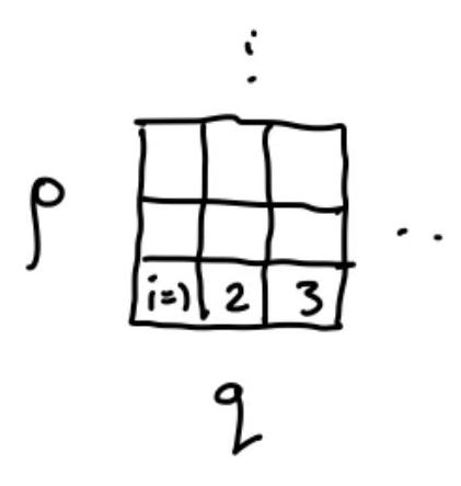
We can then coarse-grain \( P\left(\{ q, p \},t\right) \rightarrow P_{i}(t)\).

To obtain the coarse-grained dynamics \(\partial_{t} P_{i}(t)\), note that microscopic trajectories flow between cells.

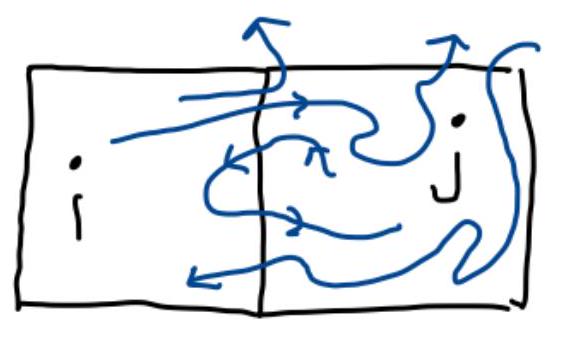
Let \(W_{j i}>0\) be the rate at which points in \(i\) go to \(j\).

So,

\[ \partial_{t} P_{i}=\underbrace{\sum_{j \neq i} W_{i j} P_{j}}_{\text{in}}-\underbrace{\sum_{j \neq i} W_{j i} P_{i}}_{\text{out}} \;. \]

This equation is called a Master equation. (Check probability conservation, \(\partial_t\sum_i P_i=0\)). The stochastic process is a “continuous-time Markov process”.

Obtaining the diffusion equation from the master equation (1D)

• define \(K\left(\zeta,x\right)\equiv W_{x+\zeta, x}\) to be the rate a trajectory currently at \(x\) jumps a distance \(\zeta\).

• assume \(K\left(\zeta,x\right)\) and \(p(x, t)\) are slowly varying in \(x\), allowing us to convert the sum into an integral.

The master equation then becomes

(21)\[ \partial_t p(x,t)=\int d\zeta \left[K(-\zeta;x+\zeta)p(x+\zeta,t)-K(\zeta;x)p(x,t)\right] \]

Note that letting \(\zeta\to -\zeta\) in the first term brings the integrand into the form \(F(-\zeta)-F(0)\) where \(F(X)\equiv K(\zeta, x+X)p(x+X,t)\). If \(F\) is slowly varying it makes sense to Taylor expand this difference,

\[ F(\zeta)-F(0) = \sum_{n=1}^{\infty} \frac{(-\zeta)^n}{n!} \partial_X^n F(X)|_{X=0}= \sum_{n=1}^{\infty} \frac{(-\zeta)^n}{n!} \partial_x^n \left(K(\zeta,x)p(x,t)\right ) \]

Inserting into (21) yields

\[ \partial_t p(x,t)=\int d\zeta \sum_{n=1}^{\infty} \frac{(-\zeta)^n}{n!} \partial_x^n \left(K(\zeta,x)p(x,t)\right ) \;. \]

Note that the integral does not involve the probability distribution itself, only the Kernel function, which is known apriori. Thus, we can perform the integrals to get the so-called Kramers-Moyal expansion

\[ \partial_t p(x,t)= \sum_{n=1}^{\infty} \frac{(-1)^n}{n!} \partial_x \left(\alpha_n(x)p(x,t)\right ) \;, \]

where

\[ \alpha_n(x)\equiv \int d\zeta \zeta^n K(\zeta,x) \]

is the \(n^{\text{th}}\) jump moment.

Diffusion limit: Only keep \(n=1,2\). The Pawula theorem shows that either all higher order moments vanish, or all even terms are positive.

Ergodic Theory

Our coarse-grained equations (master / diffusion / Kramers-Moyal) “predict”

(22)\[ P_i(t\to\infty)=P_i^{eq} \;. \]

We have seen this explicitly for the diffusion equation, provided the Stokes-Einstein relation is satisfied.

Thus, at long times, the behavior of a coarse-grained observable \(\mathcal{O}_i\) is governed by

(23)\[ \langle \mathcal{O}(t)\rangle \to \sum_i O_i P_i^{eq}=\langle \mathcal{O} \rangle_{eq} \;. \]

This means that the long-time average of any observable is identical to the ensemble average. Systems with this property are called “ergodic”.

But, clearly, our derivation was heuristic and necessarily approximate, since the coarse-grained equations break the time reversibility of the underlying dynamics (free energy is a Lyapunov function).

A more mathematically sound approach is ergodic theory.

Let \(X\) denote the microscopic state space, and for \(A \subset X, \mu(A)\) the “volume” (measure) of \(A\). E.g. for our the phase space of particles, we have

\[ \mu(A)=\int_{A} \prod_i d^{3} q_{i} \prod_j d^{3} q_{j}=\int_{A} d \mu \]

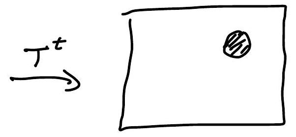
A (reversible) time evolution is a map

\[\begin{split} \begin{aligned} T^{t}: X & \rightarrow X \\ T^{t_{1}} \cdot T^{t_{2}} & =T^{t_{1}+t_{2}} \end{aligned} \end{split}\]

\(t \in \mathbb{R}^{+}, \mathbb{Z}^{+}\) for real/discrete time.

Example: Hamiltonian evolution for time “t”.

Def.: A map is called “measure preserving” if \(N(A)=N\left(T^{t}(A)\right)\) for all \(A, t\).

Example: By Liouville’s theorem, Hamiltonian dynamics is measure-preserving.

Def.: A measure-preserving \((X, \mu, T)\) is “ergodic” if

\[ T^{t}(A)=A \Rightarrow A=\{0\} \text { or } X \]

Examples: Consider a phase space “square”, \(\quad x=\{(p, q)\} \in[0,1]^{2}\).

Map \(1: T^{1}:(q, p) \rightarrow\left(q+\frac{1}{2}, p\right) \bmod 1\): It’s easy to find a set \(A\) such that \(T^1(A)=A\) (try!). \(\rightarrow\) not ergodic

Map \(2: T^{1}:(q, p) \rightarrow\left(q+\frac{e}{3}, p\right) \bmod 1\): Harder, but you can still find sts \(A\) such that \(T^1(A)=A\) (try!) \(\rightarrow\) not ergodic.

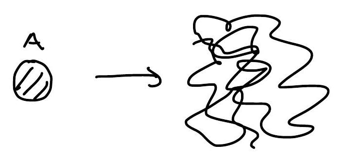
Map \(3: T^{1}:(q, p) \rightarrow\left(q+\frac{e}{3}, p+\frac{\pi}4\right) \bmod 1\): The irrationality of the shifts causes’ trajectories to “fill up” space, so \(A=\lim _{N \rightarrow \infty} \bigcup_{t=0}^{N} T^{t}\left(x_{0}\right)=X\).

Ergodic Theorem. For reasonable functions \(f\) on \(X\), ergodicity implies

\[ \lim _{N \rightarrow \infty} \frac{1}{N} \sum_{t=0}^{N} f\left(T^{t} (x_{0})\right)=\frac{1}{\mu(X)} \int_{x} f d \mu \]

(or \(\left.\frac{1}{N} \int_{t=0}^{N} f\left(T^{t} x_{0}\right) d t\right)\)

for “almost all” \(x_{0} \in X\). (exceptions have measure 0).

This is our desired property: “Average over time” \(\longrightarrow\) “average over microstates”

So, if measurements coarse grain (average) over time, we can use \(P^{eq}(x)=1/\mu(x)\)

It is interesting to note there are two distinct scenarios:

(1) Getting the ensemble average requires a long-time average over time:

(24)\[ \lim _{t \rightarrow \infty} t^{-1}\int_{t'=0}^t \int_{x} P(t', x) f(x) d \mu dt' \rightarrow \int_{x} \frac{1}{\operatorname{vol}(x)} f(x) d \mu \]

(2) At fixed time \(t \gg 0\), any initial distribution will spread out in \(X\),

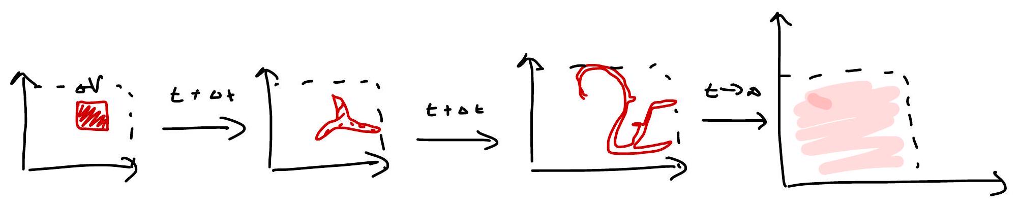
So if \(f(x)\) varies “smoothly” in \(x\),

(25)\[ \lim _{t \rightarrow \infty} \int_{x} P(t, x) f(x) d \mu \rightarrow \int_{x} \frac{1}{\operatorname{vol}(x)} f(x) d \mu \]

essentially as if \(\quad P(t \rightarrow \infty, x) \rightarrow \frac{1}{\operatorname{vol}(x)}\).

In scenario 2, regardless of how localized the initial probability distribution is, it eventually spreads across the entire state space \(X\). Consequently, the ensemble average is obtained by averaging over the probability distribution at sufficiently long times. Practically, this requires waiting for a duration significantly exceeding the system’s longest relaxation time. Note: Ergodicity implies equation (24), but not equation (25)!

Indeed, \(T:(q, p) \longrightarrow\left(q+q_{0}, p+p_{0}\right)\) is ergodic for irrational shifts, but

The mathematical property implying (2) is “mixing”:

\[ \lim _{t \rightarrow \infty} \mu\left(T^{t}(A) \cup B\right)=\mu(A) \mu(B) \]

Why? If \(T^{t}(A)\) “spreads out” evenly in space,

then since \(\mu\left(T^{t}(A)\right)=\mu(A)\), the volume of \(T^{t}(A)\) which intersects \(B\) should be proportional to \(\mu(B)\) irrespective of where \(B\) is.

Mixing is a stronger statement than ergodicity; chaotic systems are mixing.

Ergodicity has been rigorously proven for a hard sphere gas.

Application of Ergodic theory to statistical physics: the microcanonical ensemble.

Are Hamilton’s equations ergodic on phase space \(\mathbb{R}^{6 N}\) ? No! Energy is conserved, so there are invariant subsets \(\sum_{E} \in\) Phase-Space so that

\[ T^{t}\left(\Sigma_{E}\right)=\Sigma_{E} \]

However, if we restrict space to an energy shell \(\sum_E\), with measure

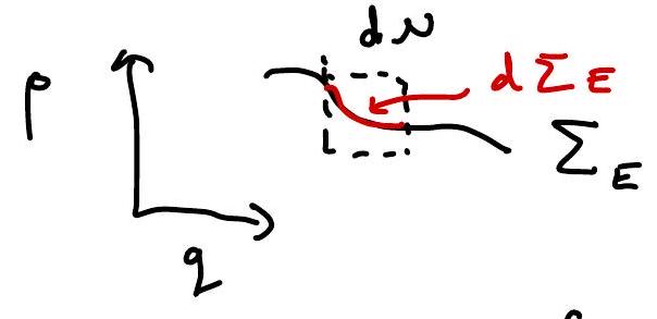
\(D(E) \cdot d \Sigma_{E} \equiv \delta(E-H(q, p)) d N\) where \(D(E) \equiv \int \delta(E-H) d_{N}\) so that \(\quad \int_{\Sigma_{E}} d \Sigma_{E}=1\), the dynamics still preserve measure \(\Sigma_{E}\).

“Ergodic hypothesis” Manybody systems are ergodic on \(\Sigma_{E}\).

So, Knowing \(E\), the coarse-grained behaviour governed by

\[ \langle f\rangle_{E} \equiv \int_{\Sigma_{E}} f \quad d \Sigma_{E} \]

We can think of this as just a particularly simple equilibrium distribution,

\[ p_{eq}(\{ q, p \}) d V=\frac{1}{D(E)} \delta(E-H(q, p )) \]

equidistributed on energy shell. The “micro canonical ensemble”.

There are fine-tuned counter examples: “integrable system”.

Also not always true if tuned to a critical point (1st order phase transitions).