
Entropy and information#
Kardar 2.7
Previously, we defined \(S \equiv \ln [\underbrace{\# \text { of configurations }}_{\Omega}](*)\). This definition is appropriate if all configurations are equally likely.
Example (Coin flipping): given \(N_{+}\) heads, the number of possible sequences with this number of heads is \(\Omega\left(N_{+}\right)=\left(\begin{array}{c}N \\ N_{+}\end{array}\right)=\frac{N !}{N_{+}! N_{-}!}\). Thus,
In general \(N_+\) is not fixed but itself a random variable with some distribution \(P\left(N_{+}\right)\), so that the entropy too is a random variable, with \(P_{S}(S) d S=P\left(N_{+}\right) d N_{+} \).
Nonetheless, from last lecture, in the thermodynamic limit we know that \(P\left(N_{+}\right)\) is sharply peaked, with
Thus,
\(\Rightarrow\) In the thermodynamic limit \((N \rightarrow \infty)\), we can only observe “typical” configurations \(\left(N_{+}=p N ; N_{-}=q N\right)\); there are \(e^{S}\) of them and all of them are equally likely, \(P(\{\sigma_i\}) = 1/e^{S} = p^{N_+} q^{N_-}\).
These observations are easily generalized to a dice with \(M\) faces. If rolling the dice results in face \(i\) with probability \(p_{i}\), we expect face \(i\) to show up exactly \(N p_i\) times in the thermodynamic limit, \(N \rightarrow \infty\). The number of typical configurations is therefore
In physics, \((*)\) arises as
the entropy change when \(M\) components are mixed together. It is therefore called “entropy of mixing”.
the entropy of system of \(N\) non-interacting subsystems. (In practice, it is enough if the subsystems are weakly interacting. For example, we can subdivide a \(1 m^3\) cube of water into \(N=10^6\) subsystems of \(cm^3-\)cubes of water. Even though there is some interaction on the interface between the small cubes, the interaction energies are negligible compared to the relevant bulk energies. In practice, it depends on a correlation length how strongly we can subdivide a given macroscopic system.) We further assume that each subsystem can be in one of \(M\) states following the probability distribution \(\{p_i\}\), i.e. a subsystem is in state \(i\) with probability \(p_i\). Then \(s=-\sum_{i=1}^M p_{i} \ln p_{i}\) is the Gibbs entropy of each of the subsystems, and \(S=N s\) is the total entropy of the system.
Interpretation as lack of knowledge#
Shannon realized that the number of possible configurations consistent with our macroscopic constraints can be viewed as a lack of knowledge about the current microstate.
Examples:
Suppose we flip coin \(N\) times and we know \(N_+\). Then, the actual microstate is one of \(e^{S\left(N_{+}\right)}\) micro-states.
If we don’t know \(N_+\), respectively \(N_+\) is not fixed? \(\Rightarrow e^{S}\) typical microstates, \(S=-N \sum_{i} p_{i} \ln p_{i}\). For a coin: \(S=-N (p \ln p +q \ln q)\).
Consequences:#
Coding#
Suppose we end up measuring the micro-state of our system of \(N\) coin flips or dice tosses, how many bits do we need to store this information?
For \(N \rightarrow \infty\), simply enumerate only the \(e^{S}\) typical microstates, all having same probabilities (namely \(1/e^{S}\)). This needs \(\log_{2}\left(e^{S}\right)=S \cdot \log_{2}(e)\) bits. (of course, this is not a proof, but it works because of CLT-induced measure concentration.)
Shannon thus gave an operational meaning to \(S\) in terms of “information” and the resources required to communicate an ensemble of messages, where each message represents a sequence of dice throws. Each symbol of the message represents a discrete random variable \(X\), attaining a value \(x_i\) with probability \(p_i\). To simplify notation Shannon introduced the information entropy of a discrete random variable \(X\):
The number of bits needed to convey a string of \(N\) such random numbers is \(N H(X)\) as \(N\to \infty\). In our original notation, the entropy \(S\) of a sequence of \(N\) dice throws is given by \(S=N H(\{p\}) \ln(2)\). Notice that the binary log appears in the Information entropy because Shannon cared about bits.
Note
Suppose, we would like to communicate a long stream of independent and identically-distributed random variables (i.i.d.), each drawn from the distribution \(p_i\). Our discussion above suggests that it is impossible to compress such data such that the code rate (average number of bits per symbol) is less than the Entropy of the source distribution, without it being virtually certain that information will be lost. (Shannon Source Coding Theorem)
Note:
\(H=\log (M)\) if \(p_{i}=\) const. \(=\frac{1}{M} \quad\) “naive encoding”
But \(H<\log (M)\) for any non-uniform probability distribution.
data compression practically implemented by using shorter codes for symbols that occur more frequently and longer codes for symbols that are less common.
For example, in the English language, letters like ‘e’, ‘t’, ‘a’, and ‘o’ are used much more frequently than letters like ‘z’, ‘q’, ‘x’, ‘j’. So, in a text compression scheme, it makes sense to use fewer bits to represent ‘e’ or ‘t’ than ‘z’ or ‘q’. This results in a smaller overall file size compared to using the same number of bits for every character.
\(I\left[\left\{p_{i}\right\}\right]=\log_{2} (M)-S\) measures information content of the pdf.
Concrete data compression example:
Suppose \(K=4\), \(\vec p=(\frac 12, \frac 14, \frac 18, \frac 18)^T\)
We could use a binary representation \(\rightarrow\) need 2 bits for 4 possibilities
Better is the code
\(1 \rightarrow 0\)
\(2 \rightarrow 10\)
\(3 \rightarrow 110\)
\(4 \rightarrow 111\)
note that the code word length \(\ell_i\) for symbol \(i\) is just \(\ell_i=\log_2 p_i\)
The average code word length per symbol is therefore \(\langle L\rangle/N=-\sum p_i\log_2p_i=H(X)=\frac 74<2\)
In fact, the above code can be generalized to obtain an optimal code for any source distribution, provided the messages are long enough and consist of uncorrelated symbols.
Below is the code to compute the entropy of a given text string. English text has a typical entropy rate of 3 to 3.5 bits per symbol, substantially less than \(\log_2(26)\approx 4.7\). Modify “sample_text” to compute the entropy of your favorite piece of poetry or prose.
import math
from collections import Counter

def compute_entropy(text):
    """
    Compute the Shannon entropy of a given text.

    Parameters:
    text (str): The input text.

    Returns:
    float: The Shannon entropy of the text.
    """
    # Convert text to lowercase and remove non-alphabetic characters
    text = ''.join(filter(str.isalpha, text.lower()))

    # Count the frequency of each character
    frequency = Counter(text)

    # Total number of characters
    total_characters = sum(frequency.values())

    # Compute the Shannon entropy
    entropy = -sum((freq / total_characters) * math.log2(freq / total_characters) for freq in frequency.values())

    return entropy

# Example usage
sample_text = """
The quick brown fox jumps over the lazy dog. This sentence is often used to test typewriters and fonts because it contains all the letters of the English alphabet.
"""

sample_textB = """I’ve written several times about the case for disqualifying Donald Trump via the 14th Amendment, arguing that it fails tests of political prudence and constitutional plausibility alike. But the debate keeps going, and the proponents of disqualification have dug into the position that whatever the prudential concerns about the amendment’s application, the events of Jan. 6, 2021, obviously amounted to an insurrection in the sense intended by the Constitution, and saying otherwise is just evasion or denial.

From their vantage point, any definition of “insurrection” that limits the amendment’s application to the kind of broad political-military rebellion that occasioned its original passage — to the hypothetical raising of a Trumpist Army of Northern Virginia, say, or the seizure of the U.S. Capitol by a Confederate States of Trumpist America — is an abuse of the natural meaning of the word. Such a limitation, they say, ignores all the obvious ways that lesser, less comprehensive forms of resistance to lawful authority clearly qualify as insurrectionary.

Here are a couple of examples of this argument: The Atlantic’s Adam Serwer, arguing with me and New York magazine’s Jonathan Chait; and the constitutional law professor Ilya Somin, going back and forth with his fellow legal scholar Steven Calabresi in Reason magazine.

I have a basic sympathy with Calabresi’s suggestion that the “paradigmatic example” that the drafters of the 14th Amendment had in mind should guide our understanding of its ambiguities, and since the paradigmatic example is the Civil War, in which hundreds of thousands of people were killed, a five-hour riot probably doesn’t clear the bar. (For related arguments about the perils of applying precedents from specific crises to radically different situations, see this essay from Samuel Issacharoff as well.)
"""


entropy_sample_text = compute_entropy(sample_text)
entropy_sample_textB = compute_entropy(sample_textB)

print(f"Shannon Entropy of sample_text A: {entropy_sample_text:.4f} bits/character")
print(f"Shannon Entropy of sample_text B: {entropy_sample_textB:.4f} bits/character")
Shannon Entropy of sample_text A: 4.1516 bits/character
Shannon Entropy of sample_text B: 4.1700 bits/character
Estimation:#
Suppose we want to estimate a distribution of \(X\), about which we have some partial information, e.g. we know the value of \(\langle X\rangle=\sum_{i} p_{i} X_{i}\) or \(\operatorname{var}(X)\), but not \(\left\{p_{i}\right\}\).
According to Shannon’s interpretation of entropy, the least biased probability distribution is the one that maximises \(H(X)\) given the constraints. This distribution is called the Maximum Entropy distribution. Any other distribution would pretend to have more information than is actually available (in form of the constraints).
Example:
Find the MaxEnt distribution under the constraint of a given fixed value \(\phi\) of \(\langle F(x)\rangle=\sum_{i} p_{i} F\left(x_{i}\right)\). It goes without saying that we also have to enforce the probability distribution summing up to one, \(\langle 1\rangle=\sum_{i} p_{i}=1\).
To maximize the entropy \(H=-\sum_{i} p_{i} \log p_{i}\) subject to both constraint, we use two Lagrange multipliers \(\alpha, \beta\) and maximize the Lagrangian function
Notes:
\(\beta\) is fixed by the the constraint of \(\langle F(x)\rangle=\phi\), and \(Z\) is fixed by the normalization of the probability distribution
This does not mean \(p\) is \(p^{*}\). Multiple \(\{p_i\}\) may give the same \(\langle F(x)\rangle\)
the above maps on the Boltzmann distribution if we identify \(\beta\equiv (k_{B} T)^{-1}\) and \(F=\text { Energy }\). The Boltzmann distribution can, therefore, be viewed as the Maximum Entropy distribution subject to the constraint of a given mean energy (also called internal energy).
One can add further constaints and update in light of extra knouledge.
How does this compare to the Bayesian updating rules?
Relative entropy (Kullback-Leibler (KL) divergence)#
Suppose the symbols \(X\) of a message are drawn from the distribution \(\operatorname{Pr}\left[X=x_{i}\right]=p_{i}\). But we think they are drawn from \(\operatorname{Pr}\left[X=x_{i}\right]=q_{i}\) instead, use correspondingly sized code words and, hence, do not optimally compress the message. Instead there will be discrepancy between the length \(L(N)\) of the number of bits we use, \(L(N)=-N \sum_{i} p_{i} \log q_{i} \) and the minimal number of bits, \(L_{min}(N)=-N \sum_{i} p_{i} \log p_{i}\), which is given by the entropy. The relative difference,
is called Kullback-Leibler (KL) divergence or relative entropxy. The KL divergence is always non-negative, which follows from Jensen’s inequality applied to the logarithm, \(\log(\mathbb{E}[X]) \geq \mathbb{E}[\log(X)]\), and vanishes only when the two distributions are identical. That’s why \( D_{K L}(\vec{p} \| \vec{q})\) is often treated like a distance between \(\vec p\) and \(\vec q\). However, the KL divergence is not a true distance measure as it is not symmetric and does not satisfy the triangle inequality.
Suppose we obtain samples \(\left\{X_{i}\right\}\) and want to decide whether they are drawn from \(\vec{p}\) or \(\vec{q}\). To this end, we compare the log-likelihoods for drawing the samples from either distribution,
Thus, we need \(\gtrsim D_{K L}^{-1}(\vec{p} \| \vec{q})\) samples to reliably tell that the samples are drawn from \(\vec{p}\) instead of \(\vec{q}\).
Note
When our calculations involve probability distributions of more than one random variable, as in the next section, it is sometimes challenging to keep the different conditional / joint / marginal distributions apart. Then, it is useful to use the following detailed notation
Note that conditional and joint probability are connected via
which implies Bayes theorem
Mutual information#
Recall that we can interpret \(H(X) \cong\) as lack of knowledge about \(X\). Measurements can reduce our lack of knowledge, but often we cannot measure a particular quantity \(X\) directly but only a quantity \(Y\) that is correlated with \(X\). For example, we may be interested in knowing the particular microstate of a 1d spin chain, but we can only measure the magnetization of the spin chain - the difference between up- and down-spins.
¿By how much does our lack of knowledge about \(X\) decrease when we measure \(Y\)? To address this question, let’s first assume we measure a particular value \(Y=y\). The fact that we now know the value of \(Y\) changes the entropy of \(X\) from the initial entropy \(H(X)\) of the \(X\) distribution,
to the entropy \(H(X|y)\) of the conditional probability distribution \(P(x|y)\) of \(x\) given \(y\),
Note that we do not necessarily have \(H(X|y)<H(X)\), for example if the particular measurement \(Y=y\) indicates that there is a lot of noise in \(X\).
However, if we average the negative entropy change over all possible \(y\)’s drawn from \(P_Y\) we obtain a non-negative quantity
which is called mutual information \(I(X;Y)\) between \(X\) and \(Y\). The mutual information measures how many bits of information we can learn on average about \(X\) when we measure \(Y\).
The notation “\(X;Y\)” makes it clear that the expression is symmetric (evident from the last line of the last formula): on average, measuring \(Y\) tells as much about \(X\) as measuring \(X\) tells us about \(Y\).
Recalling our discussion of Kullback-Leibler divergence, we see that the mutual information is a positive quantity unless \(X\) and \(Y\) are uncorrelated, \(P_{(X,Y)}=P_{X}\otimes P_Y\).
Interestingly, if we consider only discrete sets of possibilities, then entropies are positive (or zero), so that these equations imply the bounds \(0\leq I (X; Y) \leq H(X)\) and \(0\leq I (X; Y) \leq H(Y)\).
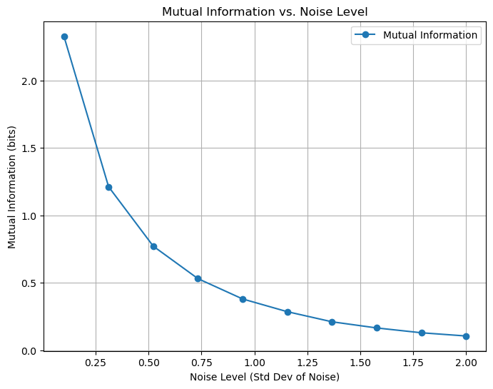
Example Mutual Information being degraded by noise#
This simple simulation illustrates how the mutual information between two random variables \( X \) and \( Y \) decays as their relationship is disturbed by noise.
Scenario#
\( X \): A random variable drawn from a normal distribution.
\( Y \): A noisy version of \( X \), where the noise level determines the correlation between \( X \) and \( Y \).
Mutual information is calculated for different levels of noise using estimation techniques.
Method#
Generate \( X \) from a standard normal distribution.
Create \( Y \) as \( Y = X + \text{noise} \), where the “noise” is a Gaussian random variable. The width of the Gaussian is varied.
Use
mutual_info_regressionfrom scikit-learn to estimate the mutual information ( I(X; Y) ).Plot the mutual information as a function of noise level.
import numpy as np
from sklearn.feature_selection import mutual_info_regression
import matplotlib.pyplot as plt

# Title and description of the notebook
"""
# Mutual Information Simulation

This notebook demonstrates the concept of mutual information using a simple example. We examine how the mutual information between two variables changes as the noise level in their relationship increases.

## Overview
- **X**: Random variable drawn from a standard normal distribution.
- **Y**: A noisy version of X.
- **Goal**: Measure the mutual information between X and Y for various noise levels.

## Libraries Used
- `numpy`: For generating random data.
- `sklearn.feature_selection`: For estimating mutual information.
- `matplotlib`: For visualization.
"""

# Parameters
n_samples = 10000  # Number of samples
noise_levels = np.linspace(0.1, 2.0, 10)  # Different noise levels
mutual_information = []

# Simulation and mutual information calculation
for noise in noise_levels:
    # Generate X from a standard normal distribution
    X = np.random.normal(0, 1, n_samples).reshape(-1, 1)
    # Generate Y as a noisy version of X
    Y = X + np.random.normal(0, noise, n_samples).reshape(-1, 1)

    # Estimate mutual information using sklearn's mutual_info_regression
    mi = mutual_info_regression(X, Y.ravel(), random_state=42)[0]
    mutual_information.append(mi)

# Visualization
plt.figure(figsize=(8, 6))
plt.plot(noise_levels, mutual_information, marker='o', linestyle='-', label="Mutual Information")
plt.title("Mutual Information vs. Noise Level")
plt.xlabel("Noise Level (Std Dev of Noise)")
plt.ylabel("Mutual Information (bits)")
plt.grid(True)
plt.legend()
plt.show()

"""
## Observations
- **Low Noise Levels**: When noise is minimal, Y closely reflects X, resulting in high mutual information.
- **High Noise Levels**: As noise increases, Y becomes less correlated with X, reducing mutual information.

## Conclusion
This simulation demonstrates how mutual information quantifies the dependence between two variables and highlights its sensitivity to noise.
"""
'\n## Observations\n- **Low Noise Levels**: When noise is minimal, Y closely reflects X, resulting in high mutual information.\n- **High Noise Levels**: As noise increases, Y becomes less correlated with X, reducing mutual information.\n\n## Conclusion\nThis simulation demonstrates how mutual information quantifies the dependence between two variables and highlights its sensitivity to noise.\n'
Observations#
Low noise: When noise is minimal, ( Y ) closely reflects ( X ), resulting in high mutual information.
High noise: As noise increases, ( Y ) becomes less correlated with ( X ), reducing mutual information.
This simulation demonstrates how mutual information quantifies the dependence between two variables, even under varying noise levels.
Information transmission#
The mutual information appears is a central quantity in information theory and appears in basic models of information flow:

\(I(X;Y)\) quantifies how efficiently \(Y\) encodes \(X\).
The maximal rate of information transmission through the channel is given by the channel capacity
Example:
To see how the ideas of entropy reduction and information work in a real example, let’s consider the response of a neuron to sensory inputs (for more, see Bialek’s book, Ch. 6.2 [Bia12] and the original paper published in PRL[SKVSB98]).
Figure 6.5 shows the results of experiments on the motion-sensitive neuron H1 in the fly visual system. In these experiments, a fly sees a randomly moving pattern, and H1 responds with a stream of spikes. If we fix \(\Delta \tau = 3\)ms nd look at \(T = 30\) ms segments of the spike train, there are \(2T /\Delta \tau \sim 10^3\) possible words, but the distribution is biased, and the entropy is only \(S(T, \Delta \tau)\sim\) 5 bits\( <\log_2(10^3)\sim 10\) bits. This relatively low entropy means that we can still sample the distributions of words even out to \(T \sim 50−60\) ms, which is interesting, because the fly can actually generate a flight correction in response to visual motion inputs within \(\sim 30\) ms.

The figure below plots
vs \(S(\text{Words})\) as a measure for how much information per second the spike trains encode about the the time stamp in the movie. The idea is that this gives an estimate of the information encoded about the entire sensory input (for which the time stamp is just a proxy).
As the time resolution \(\Delta \tau\) is varied from 800 ms down to 2 ms, the information rate follows the entropy rate \(S(\text{Words})\), with a nearly constant 50% efficiency. This result was influential because it suggests that neurons are making use of a significant fraction of their capacity in actually encoding sensory signals. Also, this is true even at millisecond time resolution. The idea that the entropy of the spike train sets a limit to neural information transmission emerged almost immediately after Shannon’s work, but it was never clear whether these limits could be approached by real systems.

Citations#
William Bialek. Biophysics: searching for principles. Princeton University Press, 2012.
Delphine Collin, Felix Ritort, Christopher Jarzynski, Steven B Smith, Ignacio Tinoco Jr, and Carlos Bustamante. Verification of the crooks fluctuation theorem and recovery of rna folding free energies. Nature, 437(7056):231–234, 2005.
Steven P Strong, Roland Koberle, Rob R De Ruyter Van Steveninck, and William Bialek. Entropy and information in neural spike trains. Physical review letters, 80(1):197, 1998.