Branching Processes

When we think about populations, one of the most basic questions is how a population grows over time from a single cell. Deterministically, we expect growth to occur if a cell is expected to produce more of itself before it dies. The expected number of offspring – the famous \(R_0\) in the context of epidemiology – has to be larger than one.

Although teproduction and death rates generally depend on age and how many offspring have already been produced, a lot of useful and generic insights can be gained by ignoring any memory. Deterministic growth then occurs when the rate \(a\) of birth exceeds the rate \(b\) of death. In fact, it is a useful excercise to show that \(R_0=a/b\), using the fact that \(a/(a+b)\) is the probability to give birth before one dies.

In many cases, birth and death rates are similar, for example in an epidemic situation where \(R_0\) is about 1, or for a slightly beneficial mutation slowly spreading in a population over time. In these near critical cases, it is not obvious whether a population survives rather than goes extinct by chance and, if it survives, what population size distribution on might expect.

N.B.: A very nice presentation of the key features of branching processes can be found in reference [DF07].

Survival probability

To answer this question, let’s first focus on the probability \(u(t|\tau)\) that an individual present at time \(\tau\) leaves some descendants at time \(t\).

Suppose, we already know \(u(t|\tau)\) and would like to estimate \(u(t|\tau-\epsilon)\), i.e. pushing the initial condition further back in time. Then, if the time slice \(\epsilon\) is sufficiently small, we only have to consider two possible events, birth with probability \(\epsilon a\), or death with probability \(\epsilon b\), as the probability of double events is of order \(\epsilon^2\). Thus, we can estimate

(1)\[ u(t|\tau-\epsilon)=\left[1-\epsilon (a+b)\right] u(t|\tau)+\epsilon a \left[1-(1-u(t|\tau))^2\right] \]

Here, the first term on the right hand side simply says that, conditional on no death or birth event occurs within the time span \(\epsilon\), the probability of survival remains unchanged.

\[ -\partial_\tau u = (a-b) u - a u^2. \]

Notice that, if the birth and death rates are time dependent, they have to be evaluated at the initial time \(\tau\). For simplicity, we assume the relative growth rate difference \(s\equiv (a-b)/a\ll1\) is constant and small.

If we further measure time in generations, \(\tau\to \tau/a\), we obtain

(2)\[ -\partial_\tau u = s u - u^2. \]

The resulting equation (2) is a logistic differential equation. Although seemingly non-linear, this equation reveals its linear nature after the following substituting \(u(\tau)=\frac {s }{1-q(\tau)^{-1}}\), upon which we obtain

\[ -\partial_\tau q(\tau)=s q(\tau) \;. \]

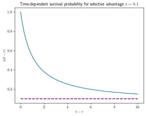
This linear equation for the fraction \(q(t)\equiv \frac u{u-s}\) has the solution \(q(\tau)=q(t)e^{s(t-\tau)}\). Using the initial condition \(q(t)=\frac 1{1-s}\), we obtain for the survival probability

\[ u(t|\tau)=\frac{s}{1-(1-s)e^{s(\tau-t)}}=u(t-\tau)\;. \]

Note, that our final result only depends on the time difference, provided that birth and death rates are time-dependent.

Note

The long-term survival probability of a super critical branching process is given by the relative growth rate difference between birth and death rate, \(s=(a-b)/a\).

Show code cell source Hide code cell source

import numpy as np
import matplotlib.pyplot as plt
# allow TeX
plt.rcParams['text.usetex'] = True
plt.figure(dpi=100)

s = 0.1
tmax = 10
t = np.linspace(start=0, stop=tmax, num=100)
y = s/(1-(1-s)*np.exp(-s*t)) 

# Add title and axis names
plt.title(r'Time-dependent survival probability for selective advantage $s = 0.1$')
plt.xlabel(r'$t- \tau $')
plt.ylabel(r'$u(t-\tau)$')

plt.hlines(y = s, xmin= 0 , xmax=tmax, colors='purple', linestyles='--', lw=2, label='s')

plt.plot(t, y)
plt.show()

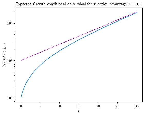
From the linear first moment equation, \(\partial_t \langle N(t)\rangle=s \langle N(t)\rangle\), it is clear that the expectation of the abundance as a function of time is a simple exponential, \(\langle N(t) \rangle =e^{st}\), which is the solution to the averaged.

But now, with the survival probability at hand, we can also predict the expected abundance given survival, because \(\langle N(t)\rangle=u(t)\langle N(t)|\text{survival} \rangle\), or

(6)\[ \langle N(t)|N(t)\geq1 \rangle =\frac{e^{st}}{u(t)}=1+\frac{e^{s t}-1}{s} \]

Show code cell source Hide code cell source

import numpy as np
import matplotlib.pyplot as plt
# allow TeX
plt.rcParams['text.usetex'] = True
plt.figure(dpi=100)

s = 0.1
tmax = 30
t = np.linspace(start=0, stop=tmax, num=100)
y = 1+(np.exp(s*t)-1)/s 

yapprox = np.exp(s*t)/s 


# Add title and axis names
plt.title(r'Expected Growth conditional on survival for selective advantage $s = 0.1$')
plt.xlabel(r'$t $')
plt.ylabel(r'$\langle N(t)|N(t)\geq1 \rangle $')

#plt.hlines(y = 1/s, xmin= 0 , xmax=tmax, colors='purple', linestyles='--', lw=2, label='s')

plt.yscale("log")

plt.plot(t, y)
plt.plot(t, yapprox, color='purple', linestyle='dashed')
plt.show()

Note

Given survival, the asymptotic exponential growth, \(s^{-1}e^{s t}\), looks as if proliferation started with \(s^{-1}\) individuals in the beginning (or earlier). This is due to accelerated growth in the beginning. Conditioned on survival, the population has to initially grow much faster than exponential, namely like \(1+t\) for a time \(s^{-1}\), to run away from the absorbing boundary.

Simulation

Let’s finally simulate a branching process and compare

Show code cell source Hide code cell source

import random
import matplotlib.pyplot as plt
import numpy as np


def simulate_branching_process(s, replicates, time_period):
    population_sizes = []
    
    for _ in range(replicates):
        population = [1]  # Start with one particle at time 0
        t = 0

        while t < time_period:
            new_population_size = np.random.poisson((1+s)*population[t])
            population.append(new_population_size)
            t += 1

        population_sizes.append(population)

    return population_sizes

s = 0.1
replicates = 50
time_period = 100

population_sizes = simulate_branching_process(s, replicates, time_period)

# Plotting the results
time_points = list(range(time_period + 1))

for i, population in enumerate(population_sizes):
    plt.plot(time_points, population)


t = np.linspace(start=0, stop=time_period, num=100)
y = 1+(np.exp(s*t)-1)/s 

yapprox = np.exp(s*t)/s 

plt.plot(t, y, color='black', linestyle='dashed', linewidth=3)
plt.plot(t, yapprox, color='purple', linestyle='dashed', linewidth=3)

plt.xlabel('Time')
plt.ylabel('Population Size')
plt.yscale("log")
plt.show()

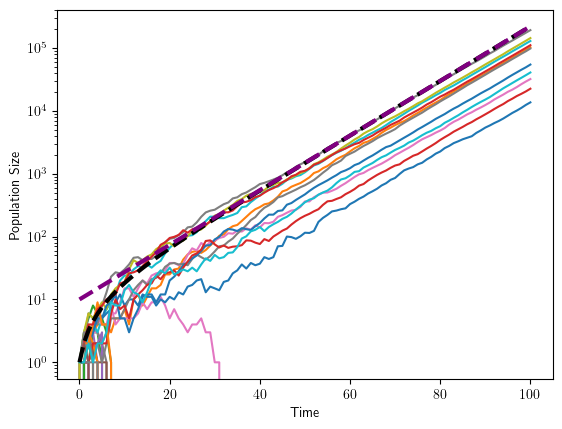
Clearly, we capture the coarse features of the process, but there are a lot of fluctuations around the expectations, even for large times.

Appendix: Population size distribution

Thus far, we have derived the survival probability of the birth-death process, but we do not know the full probability distribution \(p_n(t|\tau)\) that the population consists of \(n\) individuals at time \(t\).

But it turns out that an equation similar to the logistic equation can be derived for the moment generating function,

\[ G_x(t|\tau)\equiv \sum_{n=0}^{\infty} p_n(t|\tau) x^n \;, \]

satisfies a logistic equation very similar to the survival probability.

Retracing the steps from above, one can deduce that \(G_x(t|\tau)\) in terms of \(G_x(t|\tau-\epsilon)\),

(4)\[ G_x(t|\tau-\epsilon)=\left[1-\epsilon (a+b)\right] G_x(t|\tau)+\epsilon b +\epsilon a G_x(t|\tau)^2 \;. \]

To explain the last term on the RHS, notice that, upon birth, we have two particles and that the two-particle generating function is just the square of the one particle generating function:

\[ \sum_{n=0}^{\infty} \sum_{m=0}^{n} z^{m} p_m(t|\tau) z^{n-m} p_{n-m}(t|\tau) = \sum_{m=0}^{\infty} z^{m} p_m(t|\tau) \sum_{n-m=0}^{\infty} z^{n-m} p_{n-m}(t|\tau) =G_x(t|\tau)^2 \;. \]

In the second step, we defined \(p_{<0}(t|\tau)=0\).

In the continuous limit and after rescaling time, we find

\[ -\partial_\tau G_x = -(2-s) G_x + G_x^2 +1-s \]

First notice that we have a special solution \(G_x^\infty\equiv G_x(t-\tau\to\infty)=(1-s)\), which simply corresponds to the fact that with probability \((1-s)\) the process goes extinct (\(N(t)=0\)).

Substituting \(G_x(t)=G_x^\infty+g_x(t)\), we have to solve a logistic equation (again!)

\[ -\partial_\tau g_x = -s g_x + g_x^2 \]

subject to final condition \(x=G_x(t)=g_x(t)+1-s\), i.e., \(g_x(t)=s+x-1\), and the long-time limit \(g_x(-\infty)=0\).

This logistic differential equation can be solved for \(x\leq 1\) (indicating the radius of convergence) as above, yielding

\[ G_x(t) = 1-s+\frac{s}{1+e^{s(t-\tau)}\frac{1-x}{s+x-1}}\;. \]

A power series expansion returns the sought after abundance distribution, which for \(\tau=0\) is given by

(5)\[\begin{split} p_n(t)=\left\{\begin{array}{cc} & \begin{array}{cc} \frac{s^2 e^{s t}}{(e^{st}+s-1)(e^{st}-1)} \left(\frac{1-e^{-s t}}{1-(1-s)e^{-s t}}\right)^{n} & n\geq 1 \\ \frac{(1-s) \left(e^{s t}-1\right)}{e^{s t}+s-1} & n=0 \\ \end{array} \\ \end{array}\right. \end{split}\]

Notice that \(p_0(t)=1-u(t)\) as expected.

Since the distribution is quite broad, one would like to know some characteristic features. The mean is given by

(6)\[ \langle N(t) \rangle =\partial_x|_{x=1} G_x(t)=e^{st} \]

which again is a sanity check.

From this result, we can now compute the probability distribution, given survival. This quantity is particularly relevant for \(s t\ll 1\), where the population has established (with probability s or is extinct. In this limit, we find

(7)\[ \Pr[N(t)=n|\text{survival}]=s^{-1}p_n(t)\sim s e^{-st-ns e^{-st}} \]

This result is better interpreted by expressing the population size \(n\equiv s^{-1} e^{s(t-\Delta)}\) in terms of an effective delay time \(\Delta\) of the exponential growth period. The distribution (7) implies that this delay time follows a universal extreme value distribution,

\[ \Pr[\Delta]\propto e^{-s\Delta- e^{s\Delta}} \;, \]

the Gumbel distribution.

Show code cell source Hide code cell source

import numpy as np
import matplotlib.pyplot as plt
# allow TeX
plt.rcParams['text.usetex'] = True
plt.figure(dpi=150)


t = np.linspace(start=-3, stop=7, num=100)
y = np.exp(-t-np.exp(-t)) 

# Add title and axis names
plt.title(r'Gumbeldistribution for delay time $\Delta$')
plt.xlabel(r'$s \Delta$')
plt.ylabel(r'$\Pr[\Delta|$survival$]$')


plt.plot(t, y)
plt.show()

Citations

[BHK18]

Gabriel Birzu, Oskar Hallatschek, and Kirill S Korolev. Fluctuations uncover a distinct class of traveling waves. Proceedings of the National Academy of Sciences, 115(16):E3645–E3654, 2018.

[DF07]

Michael M Desai and Daniel S Fisher. Beneficial mutation–selection balance and the effect of linkage on positive selection. Genetics, 176(3):1759–1798, 2007.

[Hal11]

Oskar Hallatschek. The noisy edge of traveling waves. Proceedings of the National Academy of Sciences, 108(5):1783–1787, 2011.

[HG16]

Oskar Hallatschek and Lukas Geyrhofer. Collective fluctuations in the dynamics of adaptation and other traveling waves. Genetics, 202(3):1201–1227, 2016.