This page was generated from notebooks/L9/Simulating-the-diffusion-equation.ipynb.

Simulating Molecular Motors walking down a microtubule

In lecture, we discussed the evolution of the positional distribution function of a molecular motor that processively walks down a biopolymer (e.g. Kinesin V walking down a microtubule). In the simplest models, this distribution function satisfies a Smoluchowski equation of the following form. The probability density to observe the walker at position \(x\) at time \(t\) is given by

\[\partial_t p(x,t)= D \partial_x^2 p - v \partial_x p\]

where \(D\) is the diffusivity of the walker and \(v\) is its velocity.

Here, we’d like to directly time integrate the above equation to see how the pdf evolves over time.

Initializing the simulation

import numpy as np
import matplotlib.pyplot as plt

# Diffusivity of the random walkers
D = .2
# mean speed of the random walkers
v = 1.
# total length of microtubule (a.u.)
w = 40.
# simulation step size
dx = 0.01
nx = int(w/dx)
# time step of the simulation
dx2 = dx*dx
dt = dx2 / (2 * D )




uini = np.zeros(nx)
u = uini.copy()

x = np.linspace(0,w,nx)

# Initial conditions - ensemble of random walkers sharply peaked at (cx
r, cx = .2, 10
r2 = r**2
for i in range(nx):
    p2 = (i*dx-cx)**2
    if p2 < r2:
        uini[i] = 1/(2*r)

The core simulation algorithm.

def do_timestep(u0, u):
    # Propagate with forward-difference in time, central-difference in space
    u[1:-1] = u0[1:-1] + D * dt * (
          (u0[2:] - 2*u0[1:-1] + u0[:-2])/dx2 ) - v * dt * (
          (u0[2:] - u0[:-2] )/(2*dx) )

    u0 = u.copy()
    return u0, u

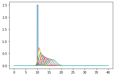
Running the simulations and plotting the output at regular time intervals

u0 = uini.copy()

# total simulation time
TotTime = 7
# Times of outputs
nsteps = 10

fig = plt.figure()
ax = fig.add_subplot(111)


for m in range(int(TotTime/dt)):
    u0, u = do_timestep(u0, u)
    if m in range(0, int(TotTime/dt), int(TotTime/(dt * nsteps))):
        ax.plot(x[1:-1], u.copy()[1:-1])

plt.show()

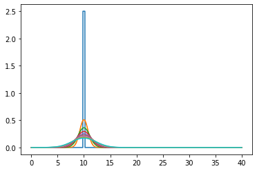
In the co-moving frame

u0 = uini.copy()

# total simulation time
TotTime = 15

# Times of outputs
nsteps = 10

fig = plt.figure()
ax = fig.add_subplot(111)


for m in range(int(TotTime/dt)):
    u0, u = do_timestep(u0, u)
    if m in range(0, int(TotTime/dt), int(TotTime/(dt * nsteps))):
        indexshift=int(v*m*dt/dx)
        ushifted=np.pad(u.copy()[indexshift:], [(0, indexshift)], mode='constant')
        ax.plot(x[1:-1], ushifted[1:-1])

plt.show()

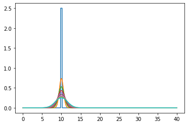
Diffusion equation without bias

Only works far away from the boundaries.

def do_timestep(u0, u):
    # Propagate with forward-difference in time, central-difference in space
    u[1:-1] = u0[1:-1] + D * dt * (
          (u0[2:] - 2*u0[1:-1] + u0[:-2])/dx2 )

    u0 = u.copy()
    return u0, u

u0 = uini.copy()

# total simulation time
TotTime = 7
# Times of outputs
nsteps = 10

fig = plt.figure()
ax = fig.add_subplot(111)


for m in range(int(TotTime/dt)):
    u0, u = do_timestep(u0, u)
    if m in range(0, int(TotTime/dt), int(TotTime/(dt * nsteps))):
        ax.plot(x[1:-1], u.copy()[1:-1])

plt.show()

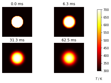
Diffusion in two dimensions

An example of a two dimensional diffusion process is the diffusion of heat from a circular source across a rectangular plate. The initial temperature is Tcold and the temperature of the heat source is Thot.

import numpy as np
import matplotlib.pyplot as plt

# plate size, mm
w = h = 10.
# intervals in x-, y- directions, mm
dx = dy = 0.1
# Thermal diffusivity of steel, mm2.s-1
D = 4.

Tcool, Thot = 300, 700

nx, ny = int(w/dx), int(h/dy)

dx2, dy2 = dx*dx, dy*dy
dt = dx2 * dy2 / (2 * D * (dx2 + dy2))

u0 = Tcool * np.ones((nx, ny))
u = u0.copy()

# Initial conditions - circle of radius r centred at (cx,cy) (mm)
r, cx, cy = 2, 5, 5
r2 = r**2
for i in range(nx):
    for j in range(ny):
        p2 = (i*dx-cx)**2 + (j*dy-cy)**2
        if p2 < r2:
            u0[i,j] = Thot

def do_timestep(u0, u):
    # Propagate with forward-difference in time, central-difference in space
    u[1:-1, 1:-1] = u0[1:-1, 1:-1] + D * dt * (
          (u0[2:, 1:-1] - 2*u0[1:-1, 1:-1] + u0[:-2, 1:-1])/dx2
          + (u0[1:-1, 2:] - 2*u0[1:-1, 1:-1] + u0[1:-1, :-2])/dy2 )

    u0 = u.copy()
    return u0, u

# Number of timesteps
nsteps = 101
# Output 4 figures at these timesteps
mfig = [0, 10, 50, 100]
fignum = 0
fig = plt.figure()
for m in range(nsteps):
    u0, u = do_timestep(u0, u)
    if m in mfig:
        fignum += 1
        print(m, fignum)
        ax = fig.add_subplot(220 + fignum)
        im = ax.imshow(u.copy(), cmap=plt.get_cmap('hot'), vmin=Tcool,vmax=Thot)
        ax.set_axis_off()
        ax.set_title('{:.1f} ms'.format(m*dt*1000))
fig.subplots_adjust(right=0.85)
cbar_ax = fig.add_axes([0.9, 0.15, 0.03, 0.7])
cbar_ax.set_xlabel('$T$ / K', labelpad=20)
fig.colorbar(im, cax=cbar_ax)
plt.show()

0 1
10 2
50 3
100 4